Asymptotic Analysis and Singular Perturbation Theory

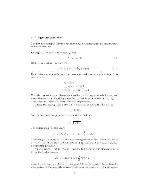
1.2 Algebraic equations
The first two examples illustrate the distinction between regular and singular perturbation
problems.
Example 1.1 Consider the cubic equation
We look for a solution of the form
x 3 − x + ε = 0. (1.2)
x = x0 + εx1 + ε 2 x2 + O(ε 3 ). (1.3)
Using this expansion in the equation, expanding, and equating coefficients of ε n to
zero, we get
x 3 0 − x0 = 0,
3x 2 0x1 − x1 + 1 = 0,
3x0x2 − x2 + 3x0x 2 1 = 0.
Note that we obtain a nonlinear equation for the leading order solution x0, and
nonhomogeneous linearized equations for the higher order corrections x1, x2,. . . .
This structure is typical of many perturbation problems.
Solving the leading-order perturbation equation, we obtain the three roots
x0 = 0, ±1.
Solving the first-order perturbation equation, we find that
The corresponding solutions are
x1 =
1
1 − 3x 2 0
x = ε + O(ε 2 ), x = ±1 − 1
2 ε + O(ε2 ).
Continuing in this way, we can obtain a convergent power series expansion about
ε = 0 for each of the three distinct roots of (1.2). This result is typical of regular
perturbation problems.
An alternative — but equivalent — method to obtain the perturbation series is
to use the Taylor expansion
x(ε) = x(0) + ˙x(0)ε + 1
2! ¨x(0)ε2 + . . . ,
where the dot denotes a derivative with respect to ε. To compute the coefficients,
we repeatedly differentiate the equation with respect to ε and set ε = 0 in the result.
3
.