Visualizing structural matrices in ANSYS using APDL - ANSYS Users

Visualizing structural matrices in ANSYS using APDL
Aaron C Acton
19 November 2008
Abstract
This article presents a method of visualizing structural matrices used in finite-element analysis using ANSYS
and the ANSYS Parametric Design Language (APDL). The information is intended to provide some insight into
the nature of structural matrices used in finite-element codes. Some terms used in sparse-matrix arithmetic are
discussed, and methods for calculating certain quantities are provided. A test model is constructed to demonstrate
how the stiffness, mass, and damping matrices may be visualized for various systems. The effect of element
shape, element type (including superelements), element reordering, and equation reordering on structural matrices
is briefly investigated.
Keywords: Potting matrices, APDL, HBMAT, Ill conditioning, Matrix condition
Tested in: ANSYS 11.0
1 Introduction
Modern finite-element codes have become advanced
tools that largely remove the user from internal calculations,
but some users may be interested to learn more
about the nature of the mathematics performed by the
code. The main purpose of this article is to provide
a visualization of some of the matrices used during the
solution of a structural finite-element analysis with AN-
SYS. Where appropriate, a brief note about a variety
of topics will be presented to aid in the explanation of
the images. All input files used to produce the images
have been provided in the appendices.
2 Graphical Output of Structural Matrices
ANSYS offers two methods of writing the structural
matrices to a plain-text file; the first method uses the
HBMAT command in the /AUX2 processor, while the second
uses a debugging option in the Solve_Info field
of the BCSOPTION command. Matrix information obtained
with HBMAT is written according to the Harwell-
Boeing standard, a general format that takes advantage
of the sparseness of typical structural matrices. Details
of the standard, in addition to several examples, were
presented by Duff, Grimes, and Lewis [1].
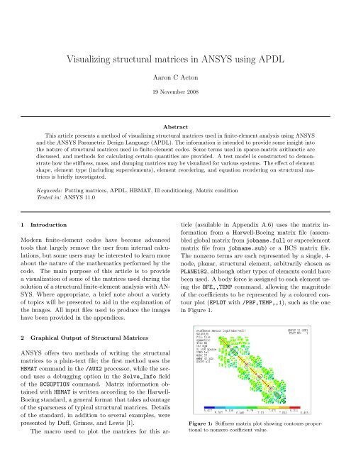
The macro used to plot the matrices for this ar-
ticle (available in Appendix A.6) uses the matrix information
from a Harwell-Boeing matrix file (assembled
global matrix from jobname.full or superelement
matrix file from jobname.sub) or a BCS matrix file.
The nonzero terms are each represented by a single, 4node,
planar, structural element, arbitrarily chosen as
PLANE182, although other types of elements could have
been used. A body force is assigned to each element using
the BFE,,TEMP command, allowing the magnitude
of the coefficients to be represented by a coloured contour
plot (EPLOT with /PBF,TEMP,,1), such as the one
in Figure 1.
Figure 1: Stiffness matrix plot showing contours proportional
to nonzero coefficient value.

A. C. Acton / Visualizing structural matrices in ANSYS using APDL 2
Since the magnitudes of the coefficients can vary by
many orders of magnitude, a logarithmic plot was obtained
by taking the base-10 logarithm of the absolute
value of each coefficient, log 10(abs(val)).
The following information was added to each plot:
• matrix type (stiffness, damping, mass),
• element type with keyoptions where appropriate,
• matrix file,
• matrix symmetry,
• number of nonzero terms (NZ),
• number of equations (EQN),
• matrix sparseness (% Sparse), and
• matrix condition number (COND).
Furthermore, if the effect of element sorting was of interest
(discussed in Section 6), the following was added:
• element sorting direction (WSORT),
• maximum wavefront (WMAX), and
• root-mean-square wavefront (WRMS).
Alternatively, if the effect of equation reordering was
of interest (discussed in Section 7), the following was
added:
• equation reordering scheme.
The meaning of these terms is discussed in the following
sections.
2.1 Number of Nonzero Terms
While the frontal solver uses the full stiffness matrix to
perform Gaussian elimination, the Boeing Sparse solver
was designed to handle only the nonzero entries, taking
advantage of the fact that structural matrices are typically
sparsely populated [2]. In addition, many structural
problems result in matrices that are symmetric
about the diagonal, allowing for further optimization
of the solution algorithms. When the system equations
are symmetric, only one triangular portion of the matrices
need to be stored. Consequently, the output from
HBMAT may contain only half of the off-diagonal terms.
The output from the HBMAT command may not accurately
report the number of nonzero terms in the
matrix; when dumping matrix information from the
jobname.sub file, all terms in the full matrix are written,
including the zero term. For this reason, the macro
provided with this article removes the nonzero terms
from the array of numerical values, then counts the
number of diagonal and off-diagonal terms. When the
matrix is symmetric, the number of nonzero terms in
the full matrix is calculated as
NNZ = 2 × ODNZ + DINZ ,
where ODNZ is the number of off-diagonal nonzero
terms and DINZ the number of diagonal nonzero terms.
Otherwise, in the case of an unsymmetric matrix,
NNZ = ODNZ + DINZ .
The nonzero terms reported by the supplied macro in
this article represents the total number of nonzero terms
in the full matrix.
2.2 Number of Equations
There will generally be more degrees of freedom (DOF)
in a model than equations in the system since some may
be condensed out before the matrices are written with
HBMAT. The following situations indicate when certain
DOF are not written to the matrix file with HBMAT:
• When constraints (D) are specified in the model,
the rows and columns corresponding to these
DOF are eliminated from the system of equations.
• When coupled sets (CP) and/or constraint equations
(CE) are present, the rows and columns corresponding
to the slave DOF are eliminated from
the system of equations.
The number of equations reported by the macro provided
with this article is simply the number of rows in
the file written with HBMAT.
2.3 Matrix Sparseness
Since typical structural matrices are said to be sparse,
it may be of interest to calculate some measure of the
sparseness, which is generally represented by the percentage
of zero terms in the matrix. Using the definition
of NNZ in section 2.1, the sparseness is calculated as
sparseness =
or, since the matrix is square,
sparseness =
NNZ
1 −
× 100% ,
NROW × NCOL
1 − NNZ
NROW2
× 100% ,
where NROW and NCOL are the number of rows and
columns reported by HBMAT, respectively.

A. C. Acton / Visualizing structural matrices in ANSYS using APDL 3
2.4 Matrix Condition
The condition number of a matrix is a measure of how
sensitive a solution is to numerical errors. A matrix
with a condition number close to unity is said to be well
conditioned, while that with a large condition number is
said to be ill conditioned. This topic has been covered
elsewhere [3].
The condition number can be computed in several
different ways, but the method used by the macro provided
with this article calculates the ratio of largest to
smallest pivot values (known as the condition number
in the two-norm), which can be obtained directly from
the jobname.DIAG file.
3 Finite Element Test Model
Since the effect of geometry on the matrix structure
was not of interest in this article, the rectangular block
shown in Figure 2 was used for all tests. In most
cases, the geometry was meshed with hexahedrons,
while tetrahedrons were used in others (images shown
later).
Figure 2: Rectangular volume used for test models.
Three faces of the volume were constrained normal
to the surface, and one of these faces was constrained for
non-structural degrees of freedom (see Appendix A.1).
When used in a substructuring analysis, all DOF for
external nodes were selected as masters. While additional
details on substructuring can be found in the
Advanced Analysis Techniques Guide [4], a short note
on substructuring is included here.
3.1 Substructuring
A substructure analysis (ANTYPE,SUBSTR) uses a technique
to reduce the system matrices to a smaller set of
DOF [2]. Internal DOF that have no applied loads or
boundary conditions, and those that will not be coupled
to other parts of the model, are condensed out of
the system matrices. As described by Bathe, “a substructure
is used in the same way as an individual finite
element with internal degrees of freedom that are statically
condensed out prior to the element assemblage
process” [5]. It is expected, then, that the substructure
matrix has less DOF and is more densely populated
than the assembled global matrix.
4 Matrix Type
The macro provided in this article supports the plotting
of real-value coefficients for stiffness, damping,
consistent-mass, and lumped-mass matrices from the
Harwell-Boeing file or from the BCS file. In the following
sections, the structure of these matrices will be
investigated.
The stiffness matrix is perhaps the most interesting
to investigate as the effect of element shape and element
type can be immediately seen.
4.1 Stiffness Matrix
Depending on the shape of the geometry being meshed,
one may decide to choose either hexahedrons (also
called bricks), tetrahedrons (also called tets), or some
combination thereof, filling in nonconformities with
prisms and pyramids where necessary. The mesh and
stiffness matrix for a simple model consisting purely of
hexahedrons can be seen in Figure 3.
Figure 3: Mesh and associated stiffness matrix for hexahedral
elements.

A. C. Acton / Visualizing structural matrices in ANSYS using APDL 4
In contrast, Figure 4 shows the mesh and stiffness
matrix for the same geometry meshed with tetrahedrons
(element edge length kept constant).
Figure 4: Mesh and associated stiffness matrix for tetrahedral
elements.
It is worth noting here that using tets in place of
bricks with equal element edge length has a significant
effect on the number of nonzero terms. In addition, the
estimated maximum value for wavefront size increased
from 57 to 87 for this model (the topic of wavefront will
be discussed further in Section 6).
If the brick model is solved as a regular superelement
(Guyan reduction) with master DOF set according
to the specifications described in Section 3, the resulting
stiffness matrix becomes dense, as shown in Figure
5.
Figure 5: Stiffness matrix for regular (Guyan reduction)
superelement.
The number of nonzero terms increases substantially,
and the number of equations decreases, causing
the sparseness to drop to near zero. The estimated
wavefront has also increased significantly.
Using component-mode synthesis (CMS) rather
than Guyan reduction results in the stiffness matrix
shown in Figure 6.
Figure 6: Stiffness matrix for CMS superelement.
Here, the sparseness increases over that for regular
superelements, for which the “tail” in the lower-right
corner is largely responsible.
4.2 Mass Matrix
The typical formation of the structural mass matrix in
implicit analyses creates coupling between degrees of
freedom. This is known as consistent mass, and can be
seen in Figure 7.
Figure 7: Consistent-mass matrix from the FULL file.
Alternatively, it may be desirable to diagonalize the
mass matrix by concentrating the mass at the nodes
(LUMPM,ON), such as in the case of a transient analysis
using explicit time integration, for which an inexpensive
matrix inversion is highly beneficial. The effect

A. C. Acton / Visualizing structural matrices in ANSYS using APDL 5
of this diagonalization becomes immediately apparent
when the mass matrix is plotted with the lumping option
turned on, as shown in Figure 8.
Figure 8: Lumped-mass matrix from the FULL file.
It should be noted here that the wavefront quantities
reported on these plots apply only to the stiffness
matrix.
Users familiar with Workbench Simulation may observe
that scoping a Point Mass feature to a large number
of nodes may require a large amount of memory
for the solution. The reason for this becomes apparent
when the mass matrix is plotted for such a model (see
Figure 9).
Figure 9: Consistent-mass matrix from the FULL file
when using the Point Mass feature in Workbench Simulation.
Additional terms appear in the mass matrix to account
for the coupling between the point mass and the
nodes to which it is attached. Two workarounds for
this issue are to turn on lumped-mass approximation
(to reduce the mass matrix to the diagonal form) or
to reduce the size of geometry to which the feature is
scoped (to reduce the number of nodes included in the
feature).
4.3 Damping Matrix
Damping is discussed last here as it is typically a factor
of one or both of the stiffness and mass matrices.
Figure 10: Alpha-damping matrix from the FULL file.
Figure 11: Beta-damping matrix from the FULL file.
Since alpha damping (ALPHAD) is a mass-matrix
multiplier, it can be seen in Figure 10 that the dampingmatrix
plot resembles the structure of the mass matrix.
[C] = α[M]
Similarly, since beta damping (BETAD) is a stiffnessmatrix
multiplier, it can be seen in Figure 11 that
the damping-matrix plot resembles the structure of the
mass matrix.
[C] = β[K]
Other forms of damping, such as modal damping,
damping ratio, and damping obtained with speciality
elements, may produce different plots than the ones
shown above.

A. C. Acton / Visualizing structural matrices in ANSYS using APDL 6
5 Element Type
The SOLID185 offers a two formulations applicable for
general finite-stain deformation. The default puredisplacement
formulation (KEYOPT(6)=0), used for simulating
compressible materials, solves the standard
static system of equations
[K]{u} = {F }
and forms the stiffness matrix shown in Figure 12.
Figure 12: Stiffness matrix for pure-displacement element
formulation.
The mixed u-P formulation (KEYOPT(6)=1), typically
used for simulating nearly-incompressible elastoplastic
or fully-incompressible hyperelastic materials,
uses a stiffness matrix of the form
[Kuu] [KuP ]
[KP u] [KP P ]
{u}
{ ¯ P }
=
{F }
{0}
and forms the stiffness matrix shown in Figure 13.
Figure 13: Stiffness matrix for mixed u-P element formulation.
Note that the condition number (discussed in Section
2.4) for the pure formulation in this example is
,
close to unity whereas that for the mixed formulation
jumps to 10 13 , indicating an ill-conditioned matrix.
This likely explains the requirement that a direct solver
must be used for the mixed formulation [6]. Also, the
number of equations increased due to the inclusion of
the hydrostatic pressure.
It is also possible to look at the structural matrices
for some coupled-field elements. The static coupled
equations for a piezoelectric element, for example, is
given by
[K] [K Z ]
[K Z ] T −[K d ]
{u}
{V }
=
{F }
{L}
which produces the symmetric stiffness matrix shown
in Figure 14. (Note that SOLID226 are quadratic elements,
whereas the SOLID185 used earlier were linear
elements, accounting for some of the extra equations.)
Figure 14: Stiffness matrix for piezoelectric elements.
In contrast, the static strongly-coupled equations
for thermoelastic elements is given by
[K] [K ut ]
[0] [K t ]
{u}
{T }
=
{F }
{Q}
which produces the unsymmetric stiffness matrix shown
in Figure 15.
,
,

A. C. Acton / Visualizing structural matrices in ANSYS using APDL 7
Figure 15: Stiffness matrix for thermoelastic elements.
Note that the weakly-coupled formulation would
produce a symmetric matrix.
6 Element Reordering
While the performance of the frontal solver
(EQSLV,FRONT) has been surpassed by the multi-frontal
design of the Sparse solver (EQSVL,SPARSE), it is instructive
to study the frontal solver as it employs the
relatively straightforward solution technique of Gaussian
elimination. During the solution of a system, the
number of equations active at any one time is called
the wavefront [2]. Before solvers included automatic
element reordering algorithms, it was important to
manually order the elements in an attempt to minimize
the maximum wavefront (representative of the amount
of memory needed for the solution) and the square of
the mean wavefront (representative of the computertime
required for the solution). The ANSYS Theory
Reference explains:
To reduce the maximum wavefront size, the
elements must be ordered so that the element
for which each node is first mentioned
is as close as possible in sequence to the element
for which it is mentioned last. In
geometric terms, the elements should be ordered
so that the wavefront sweeps through
the model continuously from one end to the
other in the direction which has the largest
number of nodes [2].
An unsorted mesh of hexahedrons may create a stiffness
matrix like the one in Figure 16, which shows a
maximum wavefront of 73.
Figure 16: Unsorted matrix for hex mesh.
One technique of reordering the elements is to use
geometric sorting (WSORT), for which a sorting direction
can be manually specified. The present topic of plotting
matrices provides an opportunity to see the effect
of sorting.
Figure 17: Location numbers of the elements in the solution
sequence and resulting stiffness matrix for sorting in
the y direction.
The concept of sorting can be thought of as the
number of equations that the solver must handle at
one time, represented graphically by a plane moving
through space. When the geometry is simple, as in
these examples, it can easily be seen that the area is
maximized when projected onto the x-z plane. The
computed maximum wavefront when sorting this model
in the y-direction is 90, which can be seen in Figure 17.

A. C. Acton / Visualizing structural matrices in ANSYS using APDL 8
Figure 18: Location numbers of the elements in the solution
sequence and resulting stiffness matrix for sorting in
the z direction.
The area is smaller when projected onto the x-y
plane. The computed maximum wavefront when sorting
this model in the z-direction is 69, which can be
seen in Figure 18.
Figure 19: Location numbers of the elements in the solution
sequence and resulting stiffness matrix for sorting in
the x direction.
Finally, the area is minimized when projected onto
the y-z plane. The computed maximum wavefront
when sorting this model in the x-direction is 57, which
can be seen in Figure 19.
When using the direct frontal solver, the elements
are automatically reordered at the beginning of the
solution process to reduce the maximum wavefront
size [7].
Element reordering can easily be confused with
equation reordering as they are both techniques used
to improve the computational efficiency of a solution;
however, the former is a technique used by the frontal
solver whereas the latter by the Sparse solver.
7 Equation Reordering
Equation reordering is an important part of the solution
procedure for the Sparse solver. The purpose of
equation reordering (achieved by graph partitioning) is
at least twofold [8]:
1. When more than one processor is available for the
solution, graph partitioning attempts to evenly
distribute the number of elements assigned to
each processor and attempts to minimize the
number of adjacent elements assigned to different
processors.
2. Graph partitioning attempts to reorder the equations
such that the amount of memory and time
required to solve a system of linear equations by
direct factorization methods is a minimum.
ANSYS offers several equation-reordering algorithms,
accessed by using the undocumented ropt field on the
BCSOPTION,ropt command, where ropt can be one of
MMD, METIS, SGI (only available on SGI systems in AN-
SYS 5.7), or WAVE [9]. It should be noted that element
reordering, as describe in Section 6, is performed
at the start of the ANSYS solution procedure; this
changes the order in which the elements are processed,
internally changes the assembled matrix, and as a result,
the changes are reflected in the jobname.full file.
Equation reordering, as described in this section, is performed
within the solver, after the system matrices are
assembled.
Unfortunately, due to the undocumented nature of
these equation-reordering techniques, there is only a
passing reference to these options in the ANSYS documentation
[2]. In fact, the format of the BCS matrix
file is also undocumented, so the accuracy of the interpretation
of these files by the macro provided with this
article cannot be guaranteed. Without explanation or
discussion, images of the stiffness matrices for METIS,

A. C. Acton / Visualizing structural matrices in ANSYS using APDL 9
MMD, and WAVES reordering are shown in Figures 20,
21, and 22, repectively.
Figure 20: Metis equation reordering.
Figure 21: MMD equation reordering.
Figure 22: Waves equation reordering.
8 Conclusions
Despite being somewhat of a “black box,” a finiteelement
code may be probed to reveal the structure
of matrices used for internal calculations. Using only
APDL, the user may visualize structural matrices to
gain more understanding of the effect that element
shape, element type, element reordering, and equation
reordering may have on the matrices.
References
[1] I. S. Duff, R. G. Grimes, and J. G. Lewis, “Users’
Guide for the Harwell-Boeing Sparse Matrix Collection
(Release I),” 1992.
[2] ANSYS, Inc., “Theory Reference for ANSYS and
ANSYS Workbench: ANSYS Release 11.0,” 2007.
[3] A. C. Acton, “A brief overview of the condition
number,” 2008.
[4] ANSYS, Inc., “Advanced Analysis Techniques
Guide: ANSYS Release 11.0,” 2007.
[5] K.-J. Bathe, Finite Element Procedures. Prentice
Hall, 2006.
[6] ANSYS, Inc., “Elements Reference: ANSYS Release
11.0,” 2007.
[7] ANSYS, Inc., “Modeling and Meshing Guide: AN-
SYS Release 11.0,” 2007.
[8] G. Karypis and V. Kumar, “MeTiS: A software
package for partitioning unstructured graphs, partitioning
meshes, and computing fill-reducing orderings
of sparse matrices,” 1998.
[9] G. Poole, “Ansys equation solvers: usage and guidelines,”
2002.

A ANSYS Input Files
All input files used for the examples presented in this article are included in the following sections. Header
information and page numbering has been removed to simplify copy-and-paste operations.
A.1 Input file used to build model
FINISH
/CLEAR
/RGB,INDEX,100,100,100,0
/RGB,INDEX,80,80,80,13
/RGB,INDEX,60,60,60,14
/RGB,INDEX,0,0,0,15
/GFILE,512
! valid only when plotting from BCS file
eqn_reord = ’MMD’ ! use "METIS", "MMD", or "WAVES"
! valid only when plotting from FULL or SUB file
sort_dir = ’all’ ! use "all", "x", "y", or "z"
matrix = ’stiff’ ! use "mass", "damp", or "stiff"
matname = ’Stiffness Matrix’ ! title to appear at top of plot
width = 5e-3
height = 2e-3
depth = 3e-3
*GET,jobname,ACTIVE,0,JOBNAM
/DELETE,%jobname%,’DIAG’
/DELETE,%matrix%,’matrix’
/DELETE,’BCS_MATRIX’,’ASCII’
/PREP7
/UNITS,SI
/VIEW,,1,2,3
!element = ’SOLID226,11’
element = ’SOLID185’
ET,1,SOLID185
!ALPHAD,5
!BETAD,0.005
!LUMPM,ON
!MAT,1
!MSHAPE,1
! steel
MP,EX,1,2E11
MP,NUXY,1,0.3
MP,DENS,1,7800
MP,KXX,1,43
! piezoelectric ceramic
MP,DENS,2,7500
MP,PERX,2,804.6
MP,PERZ,2,659.7
TB,PIEZ,2
TBDATA,16,10.5
TBDATA,14,10.5
TBDATA,3,-4.1
TBDATA,6,-4.1
TBDATA,9,14.1
TB,ANEL,2
TBDATA,1,13.2E10,7.1E10,7.3E10
TBDATA,7,13.2E10,7.3E10
TBDATA,12,11.5E10
TBDATA,16,3.0E10
TBDATA,19,2.6E10
TBDATA,21,2.6E10
BLOCK,0,width,0,height,0,depth
ESIZE,1e-3

VMESH,ALL
NSEL,S,LOC,X
D,ALL,UX,,,,,TEMP,VOLT
NSEL,S,LOC,Y
D,ALL,UY
NSEL,S,LOC,Z
D,ALL,UZ
NSEL,ALL
!/PNUM,LOC,1
!NOORDER
WSORT,%sort_dir%,,,,1E6
!/SHOW,PNG
!EPLOT
!/SHOW,CLOSE
!/SHOW,TERM
WFRONT
*GET,w_max,ACTIVE,0,WFRONT,MAX
*GET,w_rms,ACTIVE,0,WFRONT,RMS
FINISH
! README
!
! If plotting from HB file, choose either the FULL file (f2hb) or the
! SUB file (s2hb), then run hb2mat and mat2plot
!
! If plotting from BCS file, run only bm2mat and mat2plot
f2hb,matrix
!s2hb,matrix
hb2mat,matrix
!bm2mat,eqn_reord
mat2plot
A.2 Macro used to write matrix files from FULL file (f2hb.mac)
! full2hb.mac
!
! macro to write structural matrices from FULL file
!
! arguments
! 1 - matrix file to dump (stiff, damp, or mass)
/SOLU
!ANTYPE,MODAL
!MODOPT,QRDAMP,1
BCSOPT,,,,,,-1
SOLVE
FINISH
/AUX2
FILE,,full
HBMAT,%arg1%,,,ASCII,%arg1%,NO,NO
FINISH
A.3 Macro used to write matrix files from SUB file (s2hb.mac)
! sub2hb.mac
!
! reads SUB matrix file, output with HBMAT
!
! arguments
! 1 - matrix file to dump (stiff, damp, or mass)
element = ’MATRIX50’
/SOLU
ANTYPE,SUBSTR
SEOPT,,3

!CMSOPT,fix,12
NSEL,S,EXT
M,ALL,ALL
NSEL,ALL
SOLVE
FINISH
/AUX2
FILE,,sub
HBMAT,arg1,,,ASCII,arg1,NO,NO
FINISH
! this is used purely to get the estimated wavefront
/PREP7
VCLEAR,ALL
ACLEAR,ALL
ET,1,MATRIX50
SE
WFRONT
*GET,w_max,ACTIVE,0,WFRONT,MAX
*GET,w_rms,ACTIVE,0,WFRONT,RMS
FINISH
A.4 Macro file used to read HB file (hb2mat.mac)
! hb2mat.mac
!
! reads Harwell-Boeing matrix file, output with HBMAT
!
! arguments
! 1 - matrix file to dump (stiff, damp, or mass)
! the header of the Harwell-Boeing file is 4 lines
header = 4
! Harwell-Boeing file line 1 contains the title
*SREAD,title,%arg1%,’matrix’,,,,1
! extract the file that matrix was generated from
from_file = STRSUB(title(1),29,9)
*SET,title
! Harwell-Boeing file line 2 contains several length parameters
*DIM,line2,ARRAY,5
*VREAD,line2(1),%arg1%,’matrix’,,,5,,,1
(5F14.0)
totcrd = line2(1) ! total number of lines excluding header
ptrcrd = line2(2) ! number of lines for pointers
indcrd = line2(3) ! number of lines for row (or variable) indices
valcrd = line2(4) ! number of lines for numerical values
rhscrd = line2(5) ! number of lines for right-hand side
*SET,line2
! Harwell-Boeing file line 3 contains some additional length parameters
*SREAD,mxtype,%arg1%,’matrix’,,3,2,1
*DIM,line3,ARRAY,5
*VREAD,line3(1),%arg1%,’matrix’,,,5,,,2
(A3,11X,4F14.0)
nrow = line3(2) ! number of rows (or variables)
ncol = line3(3) ! number of columns (or elements)
nnzero = line3(4) ! number of row (or variable) indices
neltvl = line3(5) ! number of elemental matrix entries
*SET,line3
! if the matrix is symmetric
*IF,STRSUB(mxtype(1),2,1),EQ,’S’,THEN
! set a numerical variable for easy testing later
symmetric=1
! set a string variable for display in the plot
sym_str=’symmetric’

! otherwise, if the matrix is unsymmetric
*ELSE
symmetric=0
sym_str=’unsymmetric’
*ENDIF
! read the right-hand-side information
*IF,rhscrd,GT,0,THEN
header = header+1
*SREAD,rhstyp,%arg1%,’matrix’,,,4,1
*DIM,line4,ARRAY,3
*VREAD,line4(1),%arg1%,’matrix’,,,3,,,4
(A3,11X,2F14.0)
nrhs = line4(2) ! number of right-hand sides
nrhsix = line4(3) ! number of row indices
*SET,line4
*ENDIF
! read the column pointers into a vector
index = header
*DIM,colptr,ARRAY,ptrcrd
*VREAD,colptr(1),%arg1%,’matrix’,,,ptrcrd,,,index
(F14.0)
! fix a column-pointer bug in v11 for SUB files (has no effect for FULL files)
colptr(ptrcrd) = indcrd+1
! read the row indices into a vector
index = index+ptrcrd
*DIM,rowind,ARRAY,indcrd
*VREAD,rowind(1),%arg1%,’matrix’,,,indcrd,,,index
(F14.0)
! read the numerical values (coefficients) into a vector
index = index+indcrd
*DIM,values,ARRAY,valcrd
*VREAD,values(1),%arg1%,’matrix’,,,valcrd,,,index
(F25.15)
! read the right-hand-side values into a vector
*IF,rhscrd,GT,0,THEN
index = index+valcrd
*DIM,rhsval,ARRAY,rhscrd
*VREAD,rhsval(1),%arg1%,’matrix’,,,rhscrd,,,index
(F25.15)
*ENDIF
! convert the column pointers to column indices
*DIM,colind,ARRAY,indcrd
*DO,ii,1,ncol
*DO,jj,colptr(ii),colptr(ii+1)-1
colind(jj) = ii
*ENDDO
*ENDDO
*SET,colptr
! since there is a chance of finding zero entries, collapse them out
*VOPER,nzmask,values(1),NE,0
*VMASK,nzmask(1) $ *VFUN,nzvalues,COMP,values(1)
*VMASK,nzmask(1) $ *VFUN,nzrowind,COMP,rowind(1)
*VMASK,nzmask(1) $ *VFUN,nzcolind,COMP,colind(1)
*SET,values $ *SET,rowind $ *SET,colind $ *SET,nzmask
! optionally write the information to a text file for MATLAB/Octave sparse format
!*CFOPEN,smf,txt
!*VWRITE,nzcolind(1),nzrowind(1),nzvalues(1)
!(2F14.0,D25.15)
!*CFCLOS
! for easier processing, get the diagonals
*VOPER,dimask,nzrowind(1),EQ,nzcolind(1)
*VSCFUN,dinz,SUM,dimask(1)
! and the off-diagonals
*VOPER,odmask,nzrowind(1),NE,nzcolind(1)

*VSCFUN,odnz,SUM,odmask(1)
! determine the number of nonzeros
nnz = odnz+dinz
! HBMAT written from SUB files always contains the full matrix,
! but that from FULL files does not
*IF,STRSUB(from_file,1,4),EQ,’FULL’,THEN
*IF,symmetric,EQ,1,THEN
nnz = 2*odnz+dinz
*ENDIF
*ENDIF
! build a sparse matrix to hold all of the values
! note that ANSYS stores the transpose
*DIM,sparse,ARRAY,nnz,3
*VMASK,dimask(1) $ *VFUN,sparse(1,1),COMP,nzcolind(1)
*VMASK,dimask(1) $ *VFUN,sparse(1,2),COMP,nzrowind(1)
*VMASK,dimask(1) $ *VFUN,sparse(1,3),COMP,nzvalues(1)
*IF,odnz,GT,0,THEN
*VMASK,odmask(1) $ *VFUN,sparse(dinz+1,1),COMP,nzcolind(1)
*VMASK,odmask(1) $ *VFUN,sparse(dinz+1,2),COMP,nzrowind(1)
*VMASK,odmask(1) $ *VFUN,sparse(dinz+1,3),COMP,nzvalues(1)
*IF,STRSUB(from_file,1,4),EQ,’FULL’,THEN
*IF,symmetric,EQ,1,THEN
*VMASK,odmask(1) $ *VFUN,sparse(dinz+odnz+1,1),COMP,nzrowind(1)
*VMASK,odmask(1) $ *VFUN,sparse(dinz+odnz+1,2),COMP,nzcolind(1)
*VMASK,odmask(1) $ *VFUN,sparse(dinz+odnz+1,3),COMP,nzvalues(1)
*ENDIF
*ENDIF
*ENDIF
*SET,nzvalues $ *SET,nzrowind $ *SET,nzcolind $ *SET,dimask $ *SET,odmask
! optionally write the matrix information to a text file
!*MWRITE,sparse,’matrix’,’csv’
!%G,%G,%G
! calculate the sparseness of the matrix (percentage of zero terms)
sparseness = NINT(10000*(1-nnz/nrow/ncol))/100
! read the pivot values from the DIAG file into a vector
/INQUIRE,diag,EXIST,%jobname%,DIAG
*IF,diag,EQ,1,THEN
*DIM,pivval,ARRAY,nrow
*VREAD,pivval(1),%jobname%,’DIAG’,,,nrow,,,2
(5X,E12.8)
! the matrix condition number is the max/abs(min) pivot,
! so find the absolute maximum
*VABS,,1
*VSCFUN,pivmax,MAX,pivval(1)
! the absolute minimum
*VABS,,1
*VSCFUN,pivmin,MIN,pivval(1)
! and calculate the matrix condition number
cond = 1e60
*IF,pivmin,NE,0,THEN
cond = ’1e%NINT(LOG10(pivmax/pivmin))%’
*ENDIF
*SET,pivval
*ELSE
cond = ’?’
*ENDIF
A.5 Macro file used to read BCS file (bm2mat.mac)
! bm2mat.mac
!
! reads BCS matrix file, output with BCSOPT
!
! arguments
! 1 - equation reordering method

*GET,jobname,ACTIVE,0,JOBNAM
bcs_fil = ’BCS_MATRIX’
bcs_ext = ’ASCII’
from_file = ’BCS file’
matname = ’Stiffness Matrix’
/SOLU
BCSOPT,%arg1%,,,,ASCII,-1
SOLVE
FINISH
/INQUIRE,lines,LINES,%bcs_fil%,%bcs_ext%
! BCS matrix file line 1 contains the title
*SREAD,title,%bcs_fil%,%bcs_ext%,,,,1
! BCS matrix file line 2 contains several length parameters
*DIM,line2,ARRAY,5
*VREAD,line2(1),%bcs_fil%,%bcs_ext%,,,1,,,1
(5F10.0)
indcrd = line2(2) ! number of rows
valcrd = line2(3) ! number of lines for numerical values
nrow = indcrd ! number of rows
ncol = indcrd ! number of columns
! if the matrix is symmetric
*IF,line2(1),EQ,1,THEN
! set a numerical variable for easy testing later
symmetric=1
! set a string variable for display in the plot
sym_str=’symmetric’
! calculate the total number of nonzero terms
nnz=2*valcrd-nrow
! otherwise, if the matrix is unsymmetric
*ELSE
symmetric=0
sym_str=’unsymmetric’
nnz=valcrd
*ENDIF
*SET,line2
*DIM,rowind,ARRAY,indcrd,2
*VFILL,rowind(1,1),RAMP,1,1
*VREAD,rowind(1,2),%bcs_fil%,%bcs_ext%,,,indcrd,,,2
(8F10.0)
*DIM,sparse,ARRAY,nnz,3
*VREAD,sparse(1,1),%bcs_fil%,%bcs_ext%,,jik,3,valcrd,,lines-valcrd
(2F10.0,E25.15)
*VOPER,mapping,rowind(1,1),SCAT,rowind(1,2)
*DO,ii,1,valcrd
sparse(ii,1) = mapping(sparse(ii,1))
sparse(ii,2) = mapping(sparse(ii,2))
*ENDDO
index = valcrd+1
*DO,ii,1,valcrd
*IF,sparse(ii,1),NE,sparse(ii,2),THEN
sparse(index,1) = sparse(ii,2)
sparse(index,2) = sparse(ii,1)
sparse(index,3) = sparse(ii,3)
index = index+1
*ENDIF
*ENDDO
! calculate the sparseness of the matrix (percentage of zero terms)
*VOPER,mask,sparse(1,3),NE,0
*VSCMASK,nonzeros,SUM,mask(1)
sparseness = NINT(10000*(1-nonzeros/nrow/ncol))/100
! read the pivot values from the DIAG file into a vector

INQUIRE,diag,EXIST,%jobname%,DIAG
*IF,diag,EQ,1,THEN
*DIM,pivval,ARRAY,nrow
*VREAD,pivval(1),%jobname%,’DIAG’,,,nrow,,,2
(5X,E12.8)
! the matrix condition number is the max/abs(min) pivot,
! so find the absolute maximum
*VABS,,1
*VSCFUN,pivmax,MAX,pivval(1)
! the absolute minimum
*VABS,,1
*VSCFUN,pivmin,MIN,pivval(1)
! and calculate the matrix condition number
cond = 1e60
*IF,pivmin,NE,0,THEN
cond = ’1e%NINT(LOG10(pivmax/pivmin))%’
*ENDIF
*SET,pivval
*ELSE
cond = ’?’
*ENDIF
A.6 Macro file used to plot matrices (mat2plot.mac)
! mat2plot.mac
!
! plots nonzero values of a matrix
/PREP7
/VIEW,,,,1
VCLEAR,ALL
ACLEAR,ALL
EDELE,ALL
NDELE,ALL
/UDOC,,BODY,OFF
/UDOC,,TYPE,OFF
/PLOPTS,LOGO,OFF
/PLOPTS,DATE,OFF
/TRIAD,OFF
/PBF,TEMP,,1
/GLINE,ALL,-1
/PLOPTS,INFO,3
/TLABEL,-0.93,0.87,%matname% log10(abs(val))
/TLABEL,-0.93,0.80,%element%
/TLABEL,-0.93,0.73,%from_file%
/TLABEL,-0.93,0.66,%sym_str%
/TLABEL,-0.93,0.59,%nnz% NZ
/TLABEL,-0.93,0.52,%nrow% EQN
/TLABEL,-0.93,0.45,%sparseness%% Sparse
/TLABEL,-0.93,0.38,COND %cond%
*IF,STRSUB(from_file,1,3),EQ,’BCS’,THEN
/TLABEL,-0.93,0.31,%eqn_reord% ordering
*ELSE
/TLABEL,-0.93,0.31,WMAX %w_max%
/TLABEL,-0.93,0.24,WRMS %w_rms%
/TLABEL,-0.93,0.17,WSORT %sort_dir%
*ENDIF
CSYS,0
N,1
N,nrow+1,nrow
FILL
NGEN,ncol+1,nrow+1,ALL,,,,-1
/REP
ET,1,PLANE182
TYPE,1
! "ww" is simply the width+1, used to shorten the variable name and equation
ww=nrow+1
*DO,ii,1,nnz
*IF,sparse(ii,3),NE,0,THEN
rr = sparse(ii,1)

cc = sparse(ii,2)
EN,ii,rr*ww+cc,rr*ww+cc+1,(rr-1)*ww+cc+1,(rr-1)*ww+cc
BFE,ii,TEMP,,LOG10(ABS(sparse(ii,3)))
*ENDIF
*ENDDO
!/SHOW,PNG
EPLOT
!/SHOW,CLOSE
!/SHOW,TERM
FINISH