You also want an ePaper? Increase the reach of your titles
YUMPU automatically turns print PDFs into web optimized ePapers that Google loves.
<strong>Element</strong> <strong>Tables</strong><br />
Use of <strong>Element</strong> <strong>Tables</strong> in <strong>ANSYS</strong><br />
Sheldon Imaoka<br />
Collaborative Solutions, Inc.<br />
09/14/00
Definition of <strong>Element</strong> <strong>Tables</strong><br />
• An <strong>Element</strong> Table (ETABLE) is a “spreadsheet” of<br />
element information within <strong>ANSYS</strong>. These static arrays<br />
of information can be listed, printed, or operated upon<br />
for the following purposes:<br />
– ETABLE can be used to manipulate results for postprocessing,<br />
such as plotting “factors of safety” instead of stress values<br />
– Some elements have information which is pertinent only to<br />
that element. Hence, ETABLE is needed to retrieve these<br />
values. An example is obtaining moment and shear diagrams<br />
for BEAM elements.<br />
– <strong>Element</strong> tables are static tables, so they can be used to<br />
compare different results with each other (basic element table<br />
values can be updated automatically)<br />
CSI Tip of the Week 2
Usage of ETABLE
How to Access ETABLE<br />
ETABLE commands are accessible in the following<br />
locations:<br />
“Main Menu > General Postproc > <strong>Element</strong> Table”<br />
“Main Menu > General Postproc > Plot Results”<br />
CSI Tip of the Week 4
Steps Involved in Creating ETABLEs<br />
1) Solve problem and load results set (as needed)<br />
2) Define element table(s)<br />
– “Main Menu > General Postproc > <strong>Element</strong> Table > Define<br />
Table”<br />
3) Perform operations on tables as required<br />
– “Main Menu > General Postproc > <strong>Element</strong> Table” allows<br />
summing, adding, multiplying, taking vector or cross product<br />
of tables, just to name a few examples.<br />
4) Plot or list element tables<br />
– Plotting includes contour plots, line element results plots, or<br />
vector plots in “Main Menu > General Postproc > Plot Results”<br />
CSI Tip of the Week 5
Steps to Create ETABLE<br />
1) Solve problem and load results set (as needed)<br />
– Define results coordinate system, layer for SHELL elements<br />
General Postproc > Results Summary…<br />
General Postproc > Options for Outp…<br />
CSI Tip of the Week 6
Steps to Create ETABLE (cont.)<br />
2) Define element table(s)<br />
– “Main Menu > General Postproc > <strong>Element</strong> Table > Define<br />
Table” Provide User-Defined Name<br />
Select Category<br />
Select Item<br />
CSI Tip of the Week 7
Steps to Create ETABLE (cont.)<br />
3) Perform operations on tables as required<br />
– Sum, add, multiply, take vector or cross product of tables.<br />
General Postproc > <strong>Element</strong> Table<br />
Example of Adding two element tables<br />
CSI Tip of the Week 8
Steps to Create ETABLE (cont.)<br />
4) Plot or list element tables<br />
– Plotting can be performed with or without averaging<br />
CSI Tip of the Week 9
Obtaining <strong>Element</strong>-Specific Data<br />
Look up element<br />
information in online<br />
help.<br />
There will be a section<br />
for each element<br />
entitled “Output Data”<br />
A list of elementspecific<br />
data (“Name”)<br />
will be shown with<br />
“Item” such as “SMISC”<br />
or “NMISC”<br />
CSI Tip of the Week 10
Obtaining <strong>Element</strong>-Specific Data (cont.)<br />
For this example, a user wants N12, defined as “in-plane element<br />
stress resultant” for SHELL181 in the online help. Use the<br />
information in the table “SMISC, 3” from the chart in the previous<br />
page to obtain “N12”.<br />
CSI Tip of the Week 11
Examples of ETABLE
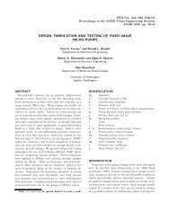
BEAM189 Example<br />
BEAM elements can be plotted with bending moment or shear<br />
force diagrams. Bending for Node I and J are noted below as<br />
SMISC,2 and SMISC,15, respectively<br />
CSI Tip of the Week 13
BEAM189 Example<br />
After defining element tables for MY for node I and J, these are<br />
plotted as “Line <strong>Element</strong> Results” as noted below:<br />
CSI Tip of the Week 14
Resulting line<br />
plot is shown<br />
at top-right.<br />
Allows for<br />
visualizing<br />
moment<br />
variation from<br />
nodes I to J for<br />
each element.<br />
Force is 100,<br />
length is 100,<br />
so we expect<br />
max moment<br />
of 10000, as<br />
noted on right.<br />
BEAM189 Example<br />
Line <strong>Element</strong> Result Plot with ETABLEs<br />
Contour plot of displacement with /ESHAPE,1<br />
CSI Tip of the Week 15
Stress resultants<br />
(force/length)<br />
can be obtained<br />
for SHELL181.<br />
Nij, Mij, and Qij<br />
are available as<br />
noted in the<br />
online help<br />
SHELL181 Example<br />
CSI Tip of the Week 16
In the online help,<br />
the “Sequence<br />
Numbers” for Nij,<br />
Mij, and Qij are<br />
listed for ETABLE<br />
definition purposes.<br />
SHELL181 Example<br />
CSI Tip of the Week 17
Resulting plot of<br />
SX and M11 for<br />
a pressureloaded<br />
plate is<br />
shown on right.<br />
SX=6*M11/t 2<br />
For this case,<br />
max SX is<br />
990638.<br />
Thickness is 0.1,<br />
so we expect<br />
M11 to be<br />
1651.06, which<br />
the obtained<br />
result.<br />
SHELL181 Example<br />
CSI Tip of the Week 18
For a given mesh,<br />
we may want to<br />
calculate<br />
volumetric<br />
properties. This<br />
may also include<br />
2D planar or<br />
axisymmetric<br />
elements.<br />
<strong>Element</strong> tables<br />
allow us to obtain<br />
volume of each<br />
element which<br />
we can then sum<br />
(SSUM command)<br />
SOLID92 Example<br />
CSI Tip of the Week 19
SOLID92 Example<br />
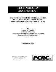
Compare solid model volume (VSUM) with volume obtained by<br />
summing each element’s volume (SSUM)<br />
CSI Tip of the Week 20
<strong>Element</strong> tables<br />
of thermal solids<br />
or thermal<br />
surface effect<br />
elements can be<br />
used to obtain<br />
heat losses due<br />
to convection<br />
(and radiation).<br />
In this example,<br />
we will look at<br />
losses due to<br />
both modes of<br />
heat transfer for<br />
SURF154<br />
SURF152 Example<br />
CSI Tip of the Week 21
SURF152 Example<br />
CSI Tip of the Week 22
SURF152 Example<br />
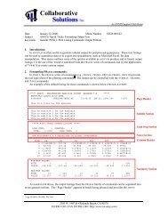
Total heat flow rate is 14.2216, which can be confirmed with<br />
reaction force (heat flow).<br />
Define element tables for heat flow rate due to convection and<br />
radiation.<br />
Sum the values to obtain totals.<br />
CSI Tip of the Week 23
SURF152 Example<br />
Results noted below. Heat loss due to convection is 8.25, due to<br />
radiation is 5.97. This adds up to 14.22, as expected for heat<br />
balance.<br />
From the results, one can conclude that radiation is a significant<br />
heat path, as posed by the problem description. (One would have<br />
done thermal resistance network to confirm this beforehand)<br />
CSI Tip of the Week 24
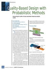
<strong>Element</strong> tables<br />
are static, so<br />
one can get<br />
element tables<br />
for different<br />
load cases (as<br />
shown on<br />
right) and<br />
compare<br />
results. With<br />
flux doubled,<br />
we expect ∆T<br />
doubled as<br />
well, which is<br />
what we get.<br />
Thermal Example<br />
CSI Tip of the Week 25
Conclusion
Additional Considerations<br />
<strong>Element</strong> tables are generally centroid values of elements. Some<br />
element tables can be a value at a given node, but only one value<br />
will be stored per element per ETABLE<br />
– For ETABLE results of DOF & other nodal quantities, these will be<br />
average of nodes of element, so min/max values will be reported<br />
lower than nodal values<br />
Parameter arrays can be inserted into ETABLE via *VPUT command<br />
– “Utility Menu > Parameters > Array Operations > Put Array Data…”<br />
Be sure to select the appropriate elements PRIOR to defining<br />
element tables, such that any calculations include only those<br />
pertinent element types<br />
– Some sequence items such as SMISC,2 or NMISC,5 mean different<br />
things for different elements. Including all elements may invalidate<br />
any further calculations.<br />
CSI Tip of the Week 27
Further References<br />
Ch. 5.2.3 “Creating an <strong>Element</strong> Table”, <strong>ANSYS</strong> 5.6 Basic<br />
Analysis Procedures Guide<br />
Ch. 2.2.2.2 “The ‘Item and Sequence Number’ Table”,<br />
<strong>ANSYS</strong> 5.6 <strong>Element</strong>s Reference<br />
“ETABLE”, <strong>ANSYS</strong> 5.6 Commands Reference<br />
CSI Tip of the Week 28