19.1 Payoff Tables and Decision Trees
19.1 Payoff Tables and Decision Trees
19.1 Payoff Tables and Decision Trees

Create successful ePaper yourself
Turn your PDF publications into a flip-book with our unique Google optimized e-Paper software.
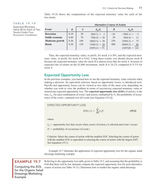
TABLE <strong>19.1</strong>0<br />
Expected Monetary<br />
Value ($) for Each of Two<br />
Stocks Under Four<br />
Economic Conditions<br />
EXAMPLE 19.7<br />
Computing the EOL<br />
for the Organic Salad<br />
Dressings Marketing<br />
Example<br />
19.2 Criteria for <strong>Decision</strong> Making 11<br />
Table <strong>19.1</strong>0 shows the computations of the expected monetary value for each of the<br />
two stocks.<br />
Thus, the expected monetary value, or profit, for stock A is $91, <strong>and</strong> the expected monetary<br />
value, or profit, for stock B is $162. Using these results, you should choose stock B<br />
because the expected monetary value for stock B is almost twice that for stock A. In terms of<br />
expected rate of return on the $1,000 investment, stock B is 16.2% compared to 9.1% for<br />
stock A.<br />
Expected Opportunity Loss<br />
In the previous examples, you learned how to use the expected monetary value criterion when<br />
making a decision. An equivalent criterion, based on opportunity losses, is introduced next.<br />
<strong>Payoff</strong>s <strong>and</strong> opportunity losses can be viewed as two sides of the same coin, depending on<br />
whether you wish to view the problem in terms of maximizing expected monetary value or<br />
minimizing expected opportunity loss. The expected opportunity loss (EOL) of action j is the<br />
loss, Lij, for each combination of event i <strong>and</strong> action j multiplied by Pi, the probability of occurrence<br />
of the event i, summed over all events [see Equation (19.2)].<br />
EXPECTED OPPORTUNITY LOSS<br />
N<br />
EOL ( j) = a LijPi i = 1<br />
where<br />
Alternative Course of Action<br />
Event Pi A Xij Pi B Xij Pi Recession 0.10 30 30(0.1) = 3 -50 -50(0.1) = -5<br />
Stable economy 0.40 70 70(0.4) = 28 30 30(0.4) = 12<br />
Moderate growth 0.30 100 100(0.3) = 30 250 250(0.3) = 75<br />
Boom 0.20 150 150(0.2) = 30 400 400(0.2) = 80<br />
EMV(A) = 91 EMV(B) = 162<br />
(19.2)<br />
Lij = opportunity loss that occurs when course of action j is selected <strong>and</strong> event i occurs<br />
Pi = probability of occurrence of event i<br />
Criterion: Select the course of action with the smallest EOL. Selecting the course of action<br />
with the smallest EOL is equivalent to selecting the course of action with the largest EMV.<br />
See Equation (<strong>19.1</strong>)<br />
Example 19.7 illustrates the application of expected opportunity loss for the organic salad<br />
dressings marketing example.<br />
Referring to the opportunity loss table given in Table 19.3, <strong>and</strong> assuming that the probability is<br />
0.60 that there will be low dem<strong>and</strong>, compute the expected opportunity loss for each alternative<br />
course of action (see Table <strong>19.1</strong>1). Determine how to market the organic salad dressings.