19.1 Payoff Tables and Decision Trees

More documents

Recommendations

Info

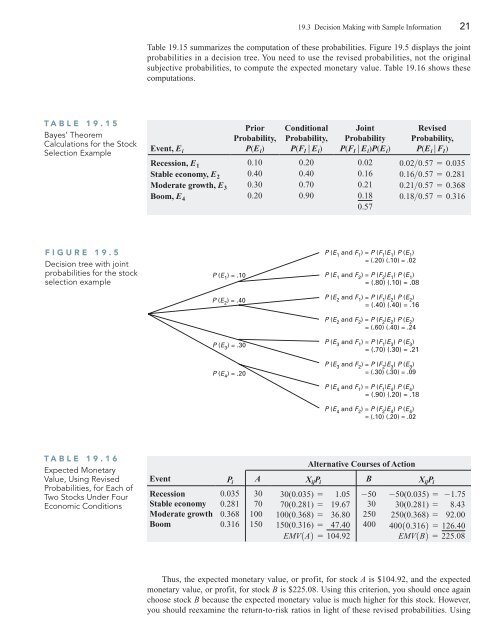
TABLE 19.15 Bayes’ Theorem Calculations for the Stock Selection Example FIGURE 19.5 Decision tree with joint probabilities for the stock selection example TABLE 19.16 Expected Monetary Value, Using Revised Probabilities, for Each of Two Stocks Under Four Economic Conditions P (E 1 ) = .10 P (E 2 ) = .40 P (E 3 ) = .30 P (E 4 ) = .20 19.3 Decision Making with Sample Information 21 Table 19.15 summarizes the computation of these probabilities. Figure 19.5 displays the joint probabilities in a decision tree. You need to use the revised probabilities, not the original subjective probabilities, to compute the expected monetary value. Table 19.16 shows these computations. Event, E i Prior Probability, P(E i) Conditional Probability, P(F 1|E i) Joint Probability P(F 1|E i)P(E i) P (E 1 and F 1 ) = P (F 1 |E 1 ) P (E 1 ) = (.20) (.10) = .02 P (E 1 and F 2 ) = P (F 2 |E 1 ) P (E 1 ) = (.80) (.10) = .08 P (E 2 and F 1 ) = P (F 1 |E 2 ) P (E 2 ) = (.40) (.40) = .16 P (E 2 and F 2 ) = P (F 2 |E 2 ) P (E 2 ) = (.60) (.40) = .24 P (E 3 and F 1 ) = P (F 1 |E 3 ) P (E 3 ) = (.70) (.30) = .21 P (E 3 and F 2 ) = P (F 2 |E 3 ) P (E 3 ) = (.30) (.30) = .09 P (E 4 and F 1 ) = P (F 1 |E 4 ) P (E 4 ) = (.90) (.20) = .18 P (E 4 and F 2 ) = P (F 2 |E 4 ) P (E 4 ) = (.10) (.20) = .02 Revised Probability, P(E i|F 1) Recession, E 1 0.10 0.20 0.02 0.02>0.57 = 0.035 Stable economy, E 2 0.40 0.40 0.16 0.16>0.57 = 0.281 Moderate growth, E 3 0.30 0.70 0.21 0.21>0.57 = 0.368 Boom, E 4 0.20 0.90 0.18 0.18>0.57 = 0.316 0.57 Alternative Courses of Action Event Pi A XijPi B XijPi Recession 0.035 30 30(0.035) = 1.05 -50 -50(0.035) = -1.75 Stable economy 0.281 70 70(0.281) = 19.67 30 30(0.281) = 8.43 Moderate growth 0.368 100 100(0.368) = 36.80 250 250(0.368) = 92.00 Boom 0.316 150 150(0.316) = 47.40 400 40010.3162 = 126.40 EMV1A2 = 104.92 EMV1B2 = 225.08 Thus, the expected monetary value, or profit, for stock A is $104.92, and the expected monetary value, or profit, for stock B is $225.08. Using this criterion, you should once again choose stock B because the expected monetary value is much higher for this stock. However, you should reexamine the return-to-risk ratios in light of these revised probabilities. Using
22 CHAPTER 19 Decision Making Equations (5.2) and (5.3) on pages 163 and 164, for stock A because EMV(A) = mA = $104.92, For stock B, because mB = $225.08, To compute the coefficient of variation, substitute s for S and EMV for X in Equation (3.8) on page 96, and s 2 N A = a (Xi - m) i = 1 2 P(Xi) = (30 - 104.92) 2 (0.035) + (70 - 104.92) 2 (0.281) + (100 - 104.92) 2 (0.368) + (150 - 104.92) 2 (0.316) = 1,190.194 s A = 11,190.194 = $34.50. s 2 N B = a (Xi - m) i = 1 2 P(Xi) = (-50 - 225.08) 2 (0.035) + (30 - 225.08) 2 (0.281) + (250 - 225.08) 2 (0.368) + (400 - 225.08) 2 (0.316) = 23,239.39 s B = 123,239.39 = $152.445. CVA = a sA b100% EMVA CVB = a sB b100% EMVB Thus, there is still much more variation in the returns from stock B than from stock A. For each of these two stocks, you calculate the return-to-risk ratios as follows. For stock A, the return-to-risk ratio is equal to RTRR(A) = 104.92 34.50 For stock B, the return-to-risk ratio is equal to = a 34.50 b100% = 32.88% 104.92 = a 152.445 b100% = 67.73% 225.08 RTRR(B) = 225.08 152.445 = 3.041 = 1.476 Thus, using the return-to-risk ratio, you should select stock A. This decision is different from the one you reached when using expected monetary value (or the equivalent expected opportunity loss). What stock should you buy? Your final decision will depend on whether you believe it is more important to maximize the expected return on investment (select stock B) or to control the relative risk (select stock A).
Page 1 and 2: 19 USING STATISTICS @ The Reliable
Page 3 and 4: 4 CHAPTER 19 Decision Making EXAMPL
Page 5 and 6: 6 CHAPTER 19 Decision Making EXAMPL
Page 7 and 8: 8 CHAPTER 19 Decision Making 19.2 C
Page 9 and 10: 10 CHAPTER 19 Decision Making EXAMP
Page 11 and 12: 12 CHAPTER 19 Decision Making TABLE
Page 13 and 14: 14 CHAPTER 19 Decision Making s for
Page 15 and 16: 16 CHAPTER 19 Decision Making b. De
Page 17 and 18: 18 CHAPTER 19 Decision Making probl
Page 19: 20 CHAPTER 19 Decision Making Becau
Page 23 and 24: 24 CHAPTER 19 Decision Making Of no
Page 25 and 26: 26 CHAPTER 19 Decision Making KEY E
Page 27 and 28: 28 CHAPTER 19 Decision Making l. If
Page 29 and 30: CHAPTER 19 EXCEL GUIDE EG19.1 PAYOF

19.1 Payoff Tables and Decision Trees

Create successful ePaper yourself

Delete template?

Save as template?