19.1 Payoff Tables and Decision Trees

19 

USING STATISTICS @ The Reliable 

Fund 

19.1 Payoff Tables and Decision 

Trees 

19.2 Criteria for Decision 

Making 

Maximax Payoff 

Maximin Payoff 

Decision Making 

Expected Monetary 

Value 

Expected Opportunity 

Loss 

Return-to-Risk Ratio 

19.3 Decision Making with 

Sample Information 

19.4 Utility 

Learning Objectives 

THINK ABOUT THIS: RISKY 

BUSINESS 

USING STATISTICS @ The Reliable 

Fund Revisited 

CHAPTER 19 EXCEL GUIDE 

In this chapter, you learn: 

• How to use payoff tables and decision trees to evaluate alternative courses 

of action 

• How to use several criteria to select an alternative course of action 

• How to use Bayes’ theorem to revise probabilities in light of sample information 

• About the concept of utility

USING STATISTICS 

@ The Reliable Fund 

As the manager of The Reliable Fund, you are responsible for purchasing and selling 

stocks for the fund. The investors in this mutual fund expect a large return on their 

investment, and at the same time they want to minimize their risk. At the present 

time, you need to decide between two stocks to purchase. An economist for your 

company has evaluated the potential one-year returns for both stocks, under four 

economic conditions: recession, stability, moderate growth, and boom. She has also estimated the 

probability of each economic condition occurring. How can you use the information provided by the 

economist to determine which stock to choose in order to maximize return and minimize risk? 

3

4 CHAPTER 19 Decision Making 

EXAMPLE 19.1 

A Payoff Table for 

Deciding How to 

Market Organic 

Salad Dressings 

In Chapter 4, you studied various rules of probability and used Bayes’ theorem to revise 

probabilities. In Chapter 5, you learned about discrete probability distributions and how to 

compute the expected value. In this chapter, these probability rules and probability distributions 

are applied to a decision-making process for evaluating alternative courses of action. In 

this context, you can consider the four basic features of a decision-making situation: 

• Alternative courses of action A decision maker must have two or more possible 

choices to evaluate prior to selecting one course of action from among the alternative 

courses of action. For example, as a manager of a mutual fund in the Using Statistics 

scenario, you must decide whether to purchase stock A or stock B. 

• Events A decision maker must list the events, or states of the world that can occur and 

consider the probability of occurrence of each event. To aid in selecting which stock to 

purchase in the Using Statistics scenario, an economist for your company has listed four 

possible economic conditions and the probability of occurrence of each event in the next 

year. 

• Payoffs In order to evaluate each course of action, a decision maker must associate a 

value or payoff with the result of each event. In business applications, this payoff is usually 

expressed in terms of profits or costs, although other payoffs, such as units of satisfaction 

or utility, are sometimes considered. In the Using Statistics scenario, the payoff is 

the return on investment. 

• Decision criteria A decision maker must determine how to select the best course of 

action. Section 19.2 discusses five decision criteria: maximax payoff, maximin payoff, 

expected monetary value, expected opportunity loss, and return-to-risk ratio. 

19.1 Payoff Tables and Decision Trees 

TABLE 19.1 

Payoff Table for the 

Organic Salad Dressings 

Marketing Example 

(in Millions of Dollars) 

In order to evaluate the alternative courses of action for a complete set of events, you need to 

develop a payoff table or construct a decision tree. A payoff table contains each possible event 

that can occur for each alternative course of action and a value or payoff for each combination 

of an event and course of action. Example 19.1 discusses a payoff table for a marketing manager 

trying to decide how to market organic salad dressings. 

You are a marketing manager for a food products company, considering the introduction of a 

new brand of organic salad dressings. You need to develop a marketing plan for the salad dressings 

in which you must decide whether you will have a gradual introduction of the salad dressings 

(with only a few different salad dressings introduced to the market) or a concentrated 

introduction of the salad dressings (in which a full line of salad dressings will be introduced to 

the market). You estimate that if there is a low demand for the salad dressings, your first year’s 

profit will be $1 million for a gradual introduction and - $5 million (a loss of $5 million) for a 

concentrated introduction. If there is high demand, you estimate that your first year’s profit will 

be $4 million for a gradual introduction and $10 million for a concentrated introduction. 

Construct a payoff table for these two alternative courses of action. 

SOLUTION Table 19.1 is a payoff table for the organic salad dressings marketing example. 

ALTERNATIVE COURSE OF ACTION 

EVENT, E i Gradual, A 1 Concentrated, A 2 

Low demand, E 1 1 -5 

High demand, E 2 4 10 

Using a decision tree is another way of representing the events for each alternative course of 

action. A decision tree pictorially represents the events and courses of action through a set of 

branches and nodes. Example 19.2 illustrates a decision tree.

EXAMPLE 19.2 

A Decision Tree for 

the Organic Salad 

Dressings Marketing 

Decision 

FIGURE 19.1 

Decision tree for the 

organic salad dressings 

marketing example (in 

millions of dollars) 

TABLE 19.2 

Predicted One-Year 

Return ($) on $1,000 

Investment in Each of 

Two Stocks, Under Four 

Economic Conditions 

FIGURE 19.2 

Decision tree for the 

stock selection payoff 

table 

19.1 Payoff Tables and Decision Trees 5 

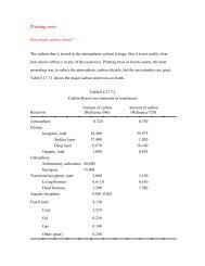
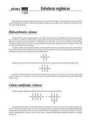
Given the payoff table for the organic salad dressings example, construct a decision tree. 

SOLUTION Figure 19.1 is the decision tree for the payoff table shown in Table 19.1. 

Gradual 

Concentrated 

Low Demand 

High Demand 

Low Demand 

High Demand 

In Figure 19.1, the first set of branches relates to the two alternative courses of action: gradual 

introduction to the market and concentrated introduction to the market. The second set of 

branches represents the possible events of low demand and high demand. These events occur 

for each of the alternative courses of action on the decision tree. 

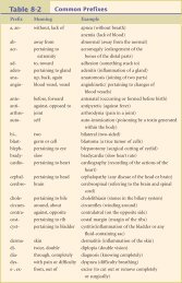
The decision structure for the organic salad dressings marketing example contains only two 

possible alternative courses of action and two possible events. In general, there can be several alternative 

courses of action and events. As a manager of The Reliable Fund in the Using Statistics scenario, 

you need to decide between two stocks to purchase for a short-term investment of one year. 

An economist at the company has predicted returns for the two stocks under four economic conditions: 

recession, stability, moderate growth, and boom. Table 19.2 presents the predicted one-year 

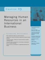
return of a $1,000 investment in each stock under each economic condition. Figure 19.2 shows the 

decision tree for this payoff table. The decision (which stock to purchase) is the first branch of the 

tree, and the second set of branches represents the four events (the economic conditions). 

STOCK 

ECONOMIC CONDITION A B 

Recession 30 -50 

Stable economy 70 30 

Moderate growth 100 250 

Boom 150 400 

Stock A 

Stock B 

$1 

$4 

–$5 

$10 

Recession 

Stable Economy 

Moderate Growth 

Boom 

Recession 

Stable Economy 

Moderate Growth 

Boom 

$30 

$70 

$100 

$150 

–$50 

$30 

$250 

$400


EXAMPLE 19.3 

Finding Opportunity 

Loss in the Organic 



TABLE 19.3 

Opportunity Loss Table 

for the Organic Salad 


Example (in Millions of 

Dollars) 

FIGURE 19.3 

Opportunity loss analysis 

worksheet results for 

Example 19.3 

Figure 19.3 displays the 

COMPUTE worksheet of the 

Opportunity Loss workbook. 

Create this worksheet using 

the instructions in Section 

EG19.1. 

You use payoff tables and decision trees as decision-making tools to help determine the 

best course of action. For example, when deciding how to market the organic salad dressings, 

you would use a concentrated introduction to the market if you knew that there would be high 

demand. You would use a gradual introduction to the market if you knew that there would be 

low demand. For each event, you can determine the amount of profit that will be lost if the best 

alternative course of action is not taken. This is called opportunity loss. 

OPPORTUNITY LOSS 

The opportunity loss is the difference between the highest possible profit for an event 

and the actual profit for an action taken. 

Example 19.3 illustrates the computation of opportunity loss. 

Using the payoff table from Example 19.1, construct an opportunity loss table. 

SOLUTION For the event “low demand,” the maximum profit occurs when there is a gradual 

introduction to the market (+ $1 million). The opportunity that is lost with a concentrated 

introduction to the market is the difference between $1 million and - $5 million, which is 

$6 million. If there is high demand, the best action is to have a concentrated introduction to 

the market ($10 million profit). The opportunity that is lost by making the incorrect decision of 

having a gradual introduction to the market is $10 million - $4 million = $6 million. The 

opportunity loss is always a nonnegative number because it represents the difference between 

the profit under the best action and any other course of action that is taken for the particular 

event. Table 19.3 shows the complete opportunity loss table for the organic salad dressings 

marketing example. 

Event 

Optimum 

Action 

Profit of 

Alternative Course of Action 

Optimum Action Gradual Concentrated 

Low demand Gradual 1 1 - 1 = 0 1 - (-5) = 6 

High demand Concentrated 10 10 - 4 = 6 10 - 10 = 0 

Figure 19.3 shows the opportunity loss analysis worksheet for Example 19.3. 

You can develop an opportunity loss table for the stock selection problem in the Using 

Statistics scenario. Here, there are four possible events or economic conditions that will affect 

the one-year return for each of the two stocks. In a recession, stock A is best, providing a return

TABLE 19.4 

Opportunity Loss Table 

($) for Two Stocks Under 

Four Economic 

Conditions 

Problems for Section 19.1 

LEARNING THE BASICS 

19.1 For this problem, use the following payoff table: 

a. Construct an opportunity loss table. 

b. Construct a decision tree. 

19.2 For this problem, use the following payoff table: 

a. Construct an opportunity loss table. 


APPLYING THE CONCEPTS 

ACTION 

EVENT A ($) B ($) 

1 50 100 

2 200 125 

ACTION 

EVENT A ($) B ($) 

1 50 10 

2 300 100 

3 500 200 

19.3 A manufacturer of designer jeans must decide 

whether to build a large factory or a small factory in a particular 

location. The profit per pair of jeans manufactured is 

estimated as $10. A small factory will incur an annual cost 

of $200,000, with a production capacity of 50,000 pairs of 

jeans per year. A large factory will incur an annual cost 

of $400,000, with a production capacity of 100,000 pairs of 

jeans per year. Four levels of manufacturing demand are 

considered likely: 10,000, 20,000, 50,000, and 100,000 pairs 

of jeans per year. 

19.1 Payoff Tables and Decision Trees 7 

of $30 as compared to a loss of $50 from stock B. In a stable economy, stock A again is better 

than stock B because it provides a return of $70 compared to $30 for stock B. However, under 

conditions of moderate growth or boom, stock B is superior to stock A. In a moderate growth 

period, stock B provides a return of $250 as compared to $100 from stock A, while in boom conditions, 

the difference between stocks is even greater, with stock B providing a return of $400 as 

compared to $150 for stock A. Table 19.4 summarizes the complete set of opportunity losses. 

Event 

Optimum 

Action 

Profit of 

Optimum 

Action 


A B 

Recession A 30 30 - 30 = 0 30 - (-50) = 80 

Stable economy A 70 70 - 70 = 0 70 - 30 = 40 

Moderate growth B 250 250 - 100 = 150 250 - 250 = 0 

Boom B 400 400 - 150 = 250 400 - 400 = 0 

a. Determine the payoffs for the possible levels of production 

for a small factory. 

b. Determine the payoffs for the possible levels of production 

for a large factory. 

c. Based on the results of (a) and (b), construct a payoff 

table, indicating the events and alternative courses of 

action. 

d. Construct a decision tree. 

e. Construct an opportunity loss table. 

19.4 An author is trying to choose between two publishing 

companies that are competing for the marketing rights to her 

new novel. Company A has offered the author $10,000 plus 

$2 per book sold. Company B has offered the author $2,000 

plus $4 per book sold. The author believes that five levels of 

demand for the book are possible: 1,000, 2,000, 5,000, 

10,000, and 50,000 books sold. 

a. Compute the payoffs for each level of demand for company 

A and company B. 

b. Construct a payoff table, indicating the events and alternative 

courses of action. 

c. Construct a decision tree. 

d. Construct an opportunity loss table. 

19.5 The DellaVecchia Garden Center purchases and sells 

Christmas trees during the holiday season. It purchases the 

trees for $10 each and sells them for $20 each. Any trees not 

sold by Christmas day are sold for $2 each to a company that 

makes wood chips. The garden center estimates that four levels 

of demand are possible: 100, 200, 500, and 1,000 trees. 

a. Compute the payoffs for purchasing 100, 200, 500, or 

1,000 trees for each of the four levels of demand. 

b. Construct a payoff table, indicating the events and alternative 


c. Construct a decision tree. 

d. Construct an opportunity loss table.


19.2 Criteria for Decision Making 

EXAMPLE 19.4 

Finding the Best 

Course of Action 

According to the 

Maximax Criterion 

for the Organic 



TABLE 19.5 

Using the Maximax 

Criterion for the 

Organic Salad 


Example (in Millions 

of Dollars) 

TABLE 19.6 

Using the Maximax 



Return ($) on $1,000 




After you compute the profit and opportunity loss for each event under each alternative course of 

action, you need to determine the criteria for selecting the most desirable course of action. Some 

criteria involve the assignment of probabilities to each event, but others do not. This section introduces 

two criteria that do not use probabilities: the maximax payoff and the maximin payoff. 

This section presents three decision criteria involving probabilities: expected monetary 

value, expected opportunity loss, and the return-to-risk ratio. For criteria in which a probability 

is assigned to each event, the probability is based on information available from past data, 

from the opinions of the decision maker, or from knowledge about the probability distribution 

that the event may follow. Using these probabilities, along with the payoffs or opportunity 

losses of each event–action combination, you select the best course of action according to a 

particular criterion. 

Maximax Payoff 

The maximax payoff criterion is an optimistic payoff criterion. Using this criterion, you do 

the following: 

1. Find the maximum payoff for each action. 

2. Choose the action that has the highest of these maximum payoffs. 

Example 19.4 illustrates the application of the maximax criterion to the organic salad 

dressings marketing example. 

Return to Table 19.1, the payoff table for deciding how to market organic salad dressings. 

Determine the best course of action according to the maximax criterion. 

SOLUTION First you find the maximum profit for each action. For a gradual introduction 

to the market, the maximum profit is $4 million. For a concentrated introduction to the market, 

the maximum profit is $10 million. Because the maximum of the maximum profits is 

$10 million, you choose the action that involves a concentrated introduction to the market. 

Table 19.5 summarizes the use of this criterion. 


EVENT, E i Gradual, A 1 Concentrated, A 2 

High demand, E 1 1 -5 

High demand, E 2 4 10 

Maximum profit for each action 4 10* 

As a second application of the maximax payoff criterion, return to the Using Statistics scenario 

and the payoff table presented in Table 19.2. Table 19.6 summarizes the maximax payoff 

criterion for that example. 

STOCK 





Boom 150 400 

Maximum profit for each action 150 400

EXAMPLE 19.5 

Finding the Best 

Course of Action 

According to the 

Maximin Criterion 

for the Organic 



TABLE 19.7 

Using the Maximin 


Organic Salad 


Example (in Millions 

of Dollars) 

TABLE 19.8 

Using the Maximin 



Return ($) on $1,000 




19.2 Criteria for Decision Making 9 

Because the maximum of the maximum profits is $400, you choose stock B. 

Maximin Payoff 

The maximin payoff criterion is a pessimistic payoff criterion. Using this criterion, you do the 

following: 

1. Find the minimum payoff for each action. 

2. Choose the action that has the highest of these minimum payoffs. 

Example 19.5 illustrates the application of the maximin criterion to the organic salad dressing 

marketing example. 

Return to Table 19.1, the payoff table for deciding how to market organic salad dressings. 

Determine the best course of action according to the maximin criterion. 

SOLUTION First, you find the minimum profit for each action. For a gradual introduction to 

the market, the minimum profit is $1 million. For a concentrated introduction to the market, the 

minimum profit is - $5 million. Because the maximum of the minimum profits is $1 million, 

you choose the action that involves a gradual introduction to the market. Table 19.7 summarizes 

the use of this criterion. 


EVENT, Ei Gradual, A1 Concentrated, A2 Low demand, E1 1 -5 

High demand, E2 4 10 

Minimum profit for each action 1 -5 

As a second application of the maximin payoff criterion, return to the Using Statistics scenario 

and the payoff table presented in Table 19.2. Table 19.8 summarizes the maximin payoff 

criterion for that example. 

STOCK 





Boom 150 400 

Minimum profit for each action 30 -50 

Because the maximum of the minimum profits is $30, you choose stock A. 

Expected Monetary Value 

The expected value of a probability distribution was computed in Equation (5.1) on page 163. 

Now you use Equation (5.1) to compute the expected monetary value for each alternative 

course of action. The expected monetary value (EMV ) for a course of action, j, is the payoff 

(Xij) for each combination of event i and action j multiplied by Pi, the probability of occurrence 

of event i, summed over all events [see Equation (19.1)].


EXAMPLE 19.6 

Computing the EMV 

in the Organic Salad 


Example 

TABLE 19.9 


Value (in Millions of 

Dollars) for Each 

Alternative for the 

Organic Salad 


Example 

EXPECTED MONETARY VALUE 

where 

N 

EMV ( j) = a XijPi i = 1 

(19.1) 

EMV ( j) = expected monetary value of action j 

Xij = payoff that occurs when course of action j is selected and event i occurs 

Pi = probability of occurrence of event i 

N = number of events 

Criterion: Select the course of action with the largest EMV. 

Example 19.6 illustrates the application of expected monetary value to the organic salad 


Returning to the payoff table for deciding how to market organic salad dressings (Example 19.1), 

suppose that the probability is 0.60 that there will be low demand (so that the probability is 0.40 

that there will be high demand). Compute the expected monetary value for each alternative 

course of action and determine how to market organic salad dressings. 

SOLUTION You use Equation (19.1) to determine the expected monetary value for each 

alternative course of action. Table 19.9 summarizes these computations. 


Event P i Gradual, A 1 X ij P i Concentrated, A 2 X ij P i 

Low demand, E 1 0.60 1 1(0.6) = 0.6 -5 -5(0.6) = -3.0 

High demand, E 2 0.40 4 4(0.4) = 1.6 10 10(0.4) = 4.0 

EMV(A 1) = 2.2 EMV(A 2) = 1.0 

The expected monetary value for a gradual introduction to the market is $2.2 million, and 

the expected monetary value for a concentrated introduction to the market is $1 million. 

Thus, if your objective is to choose the action that maximizes the expected monetary value, 

you would choose the action of a gradual introduction to the market because its EMV is 

highest. 

As a second application of expected monetary value, return to the Using Statistics scenario 

and the payoff table presented in Table 19.2. Suppose the company economist assigns the following 

probabilities to the different economic conditions: 

P(Recession) = 0.10 

P(Stable economy) = 0.40 

P(Moderate growth) = 0.30 

P(Boom) = 0.20

TABLE 19.10 


Value ($) for Each of Two 

Stocks Under Four 


EXAMPLE 19.7 

Computing the EOL 



Example 


Table 19.10 shows the computations of the expected monetary value for each of the 

two stocks. 

Thus, the expected monetary value, or profit, for stock A is $91, and the expected monetary 

value, or profit, for stock B is $162. Using these results, you should choose stock B 

because the expected monetary value for stock B is almost twice that for stock A. In terms of 

expected rate of return on the $1,000 investment, stock B is 16.2% compared to 9.1% for 

stock A. 

Expected Opportunity Loss 

In the previous examples, you learned how to use the expected monetary value criterion when 

making a decision. An equivalent criterion, based on opportunity losses, is introduced next. 

Payoffs and opportunity losses can be viewed as two sides of the same coin, depending on 

whether you wish to view the problem in terms of maximizing expected monetary value or 

minimizing expected opportunity loss. The expected opportunity loss (EOL) of action j is the 

loss, Lij, for each combination of event i and action j multiplied by Pi, the probability of occurrence 

of the event i, summed over all events [see Equation (19.2)]. 

EXPECTED OPPORTUNITY LOSS 

N 

EOL ( j) = a LijPi i = 1 

where 


Event Pi A Xij Pi B Xij Pi Recession 0.10 30 30(0.1) = 3 -50 -50(0.1) = -5 

Stable economy 0.40 70 70(0.4) = 28 30 30(0.4) = 12 

Moderate growth 0.30 100 100(0.3) = 30 250 250(0.3) = 75 

Boom 0.20 150 150(0.2) = 30 400 400(0.2) = 80 

EMV(A) = 91 EMV(B) = 162 

(19.2) 

Lij = opportunity loss that occurs when course of action j is selected and event i occurs 

Pi = probability of occurrence of event i 

Criterion: Select the course of action with the smallest EOL. Selecting the course of action 

with the smallest EOL is equivalent to selecting the course of action with the largest EMV. 

See Equation (19.1) 

Example 19.7 illustrates the application of expected opportunity loss for the organic salad 


Referring to the opportunity loss table given in Table 19.3, and assuming that the probability is 

0.60 that there will be low demand, compute the expected opportunity loss for each alternative 

course of action (see Table 19.11). Determine how to market the organic salad dressings.




Loss (in Millions of 

Dollars) for Each 

Alternative for the 

Organic Salad 


Example 

EXAMPLE 19.8 

Computing the EVPI 

in the Organic Salad 


Example 

The expected opportunity loss from the best decision is called the expected value of perfect 

information (EVPI). Equation (19.3) defines the EVPI. 

EXPECTED VALUE OF PERFECT INFORMATION 

The expected profit under certainty represents the expected profit that you could 

make if you had perfect information about which event will occur. 

EVPI = expected profit under certainty 

- expected monetary value of the best alternative 

(19.3) 

Referring to the data in Example 19.6, compute the expected profit under certainty and the 

expected value of perfect information. 

SOLUTION As the marketing manager of the food products company, if you could always 

predict the future, a profit of $1 million would be made for the 60% of the time that there is low 

demand, and a profit of $10 million would be made for the 40% of the time that there is high 

demand. Thus, 

Expected profit under certainty = 0.60($1) + 0.40($10) 

The $4.60 million represents the profit you could make if you knew with certainty what the 

demand would be for the organic salad dressings. You use the EMV calculations in Table 19.9 

and Equation (19.3) to compute the expected value of perfect information: 

EVPI = Expected profit under certainty - expected monetary value of the best alternative 

= $4.6 - ($2.2) = $2.4 


Event, E i P i Gradual, A 1 L ij P i Concentrated, A 2 L ij P i 

Low demand, E 1 0.60 0 0(0.6) = 0 6 6(0.6) = 3.6 

High demand, E 2 0.40 6 6(0.4) = 2.4 0 0(0.4) = 0 

EOL(A 1) = 2.4 EOL(A 2) = 3.6 

SOLUTION The expected opportunity loss is lower for a gradual introduction to the market 

($2.4 million) than for a concentrated introduction to the market ($3.6 million). 

Therefore, using the EOL criterion, the optimal decision is for a gradual introduction to the 

market. This outcome is expected because the equivalent EMV criterion produced the same 

optimal strategy. 

Example 19.8 illustrates the expected value of perfect information. 

= $0.60 - $4.00 

= $4.60 

This EVPI value of $2.4 million represents the maximum amount that you should be willing to 

pay for perfect information. Of course, you can never have perfect information, and you should 

never pay the entire EVPI for more information. Rather, the EVPI provides a guideline for an 

upper bound on how much you might consider paying for better information. The EVPI is also 

the expected opportunity loss for a gradual introduction to the market, the best action according 

to the EMV criterion.



Loss for Each Alternative 

($) for the Stock 

Selection Example 


Return to the Using Statistics scenario and the opportunity loss table presented in Table 

19.4. Table 19.12 presents the computations to determine the expected opportunity loss for 

stock A and stock B. 


Event P i A L ij P i B L ij P i 

Recession 0.10 0 0(0.1) = 0 80 80(0.1) = 8 

Stable economy 0.40 0 0(0.4) = 0 40 40(0.4) = 16 

Moderate growth 0.30 150 150(0.3) = 45 0 0(0.3) = 0 

Boom 0.20 250 250(0.2) = 50 0 0(0.2) = 0 

EOL(A) = 95 EOL(B) = EVPI = 24 

The expected opportunity loss is lower for stock B than for stock A. Your optimal decision 

is to choose stock B, which is consistent with the decision made using expected monetary 

value. The expected value of perfect information is $24 (per $1,000 invested), meaning that you 

should be willing to pay up to $24 for perfect information. 


Unfortunately, neither the expected monetary value nor the expected opportunity loss criterion 

takes into account the variability of the payoffs for the alternative courses of action under different 

events. From Table 19.2, you see that the return for stock A varies from $30 in a recession 

to $150 in an economic boom, whereas the return for stock B (the one chosen according to 

the expected monetary value and expected opportunity loss criteria) varies from a loss of $50 

in a recession to a profit of $400 in an economic boom. 

To take into account the variability of the events (in this case, the different economic 

conditions), you can compute the variance and standard deviation of each stock, using 

Equations (5.2) and (5.3) on pages 163 and 164. Using the information presented in Table 

19.10, for stock A, EMV(A) = mA = $91, 

and the variance is 

s 2 N 

A = a (Xi - m) 

i = 1 

2 P(Xi) = (30 - 91) 2 (0.1) + (70 - 91) 2 (0.4) + (100 - 91) 2 (0.3) + (150 - 91) 2 (0.2) 

= 1,269 

and s A = 11,269 = $35.62. 

For stock B, EMV(B) = mB = $162, and the variance is 

s 2 N 

B = a (Xi - m) 

i = 1 

2 P(Xi) = (-50 - 162) 2 (0.1) + (30 - 162) 2 (0.4) + (250 - 162) 2 (0.3) 

+ (400 - 162) 2 (0.2) 

= 25,116 

and s B = 125,116 = $158.48. 

Because you are comparing two stocks with different means, you should evaluate the relative 

risk associated with each stock. Once you compute the standard deviation of the return 

from each stock, you compute the coefficient of variation discussed in Section 3.2. Substituting


s 

for S and EMV for X in Equation (3.7) on page 93, you find that the coefficient of variation 

for stock A is equal to 

whereas the coefficient of variation for stock B is equal to 

Thus, there is much more variation in the return for stock B than for stock A. 

When there are large differences in the amount of variability in the different events, a criterion 

other than EMV or EOL is needed to express the relationship between the return (as 

expressed by the EMV) and the risk (as expressed by the standard deviation). Equation (19.4) 

defines the return-to-risk ratio (RTRR) as the expected monetary value of action j divided by 

the standard deviation of action j. 

RETURN-TO-RISK RATIO 

where 

CVA = a sA b100% 

EMVA EMV ( j) = expected monetary value for alternative course of action j 

sj = standard deviation for alternative course of action j 

Criterion: Select the course of action with the largest RTRR. 

(19.4) 

For each of the two stocks discussed previously, you compute the return-to-risk ratio as follows. 

For stock A, the return-to-risk ratio is equal to 

RTRR(A) = 91 

35.62 

For stock B, the return-to-risk ratio is equal to 

= a 35.62 

b100% = 39.1% 

91 

CVB = a sB b100% 

EMVB = a 158.48 

b100% = 97.8% 

162 

RTRR( j) = 

RTRR(B) = 162 

158.48 

EMV( j) 

s j 

= 2.55 

= 1.02 

Thus, relative to the risk as expressed by the standard deviation, the expected return is much 

higher for stock A than for stock B. Stock A has a smaller expected monetary value than stock 

B but also has a much smaller risk than stock B. The return-to-risk ratio shows A to be preferable 

to B. Figure 19.4 shows the worksheet results for this problem.

FIGURE 19.4 

Expected monetary value 

and standard deviation 

worksheet results for 

stock selection problem 

Figure 19.4 displays the 

COMPUTE worksheet of the 


workbook. Create this 

worksheet using the 

instructions in Section EG19.2. 

Problems for Section 19.2 


19.6 For the following payoff table, the probability of event 

1 is 0.5, and the probability of event 2 is also 0.5: 

ACTION 

EVENT A ($) B ($) 

1 50 100 

2 200 125 

a. Determine the optimal action based on the maximax 

criterion. 

b. Determine the optimal action based on the maximin 

criterion. 

c. Compute the expected monetary value (EMV) for actions 

A and B. 

d. Compute the expected opportunity loss (EOL) for actions 


e. Explain the meaning of the expected value of perfect 

information (EVPI) in this problem. 


f. Based on the results of (c) or (d), which action would you 

choose? Why? 

g. Compute the coefficient of variation for each action. 

h. Compute the return-to-risk ratio (RTRR) for each action. 

i. Based on (g) and (h), what action would you choose? Why? 

j. Compare the results of (f) and (i) and explain any 

differences. 

19.7 For the following payoff table, the probability of event 

1 is 0.8, the probability of event 2 is 0.1, and the probability 

of event 3 is 0.1: 

ACTION 

EVENT A ($) B ($) 

1 50 10 

2 300 100 

3 500 200 


criterion.



criterion. 

c. Compute the expected monetary value (EMV) for actions 


d. Compute the expected opportunity loss (EOL) for actions 




f. Based on the results of (c) or (d), which action would you 

choose? Why? 

g. Compute the coefficient of variation for each action. 

h. Compute the return-to-risk ratio (RTRR) for each action. 

i. Based on (g) and (h), what action would you choose? 

Why? 


differences. 

k. Would your answers to (f) and (i) be different if the probabilities 

for the three events were 0.1, 0.1, and 0.8, 

respectively? Discuss. 

19.8 For a potential investment of $1,000, if a stock has an 

EMV of $100 and a standard deviation of $25, what is the 

a. rate of return? 

b. coefficient of variation? 

c. return-to-risk ratio? 

19.9 A stock has the following predicted returns under the 

following economic conditions: 

Economic Condition Probability Return ($) 

Recession 0.30 50 

Stable economy 0.30 100 

Moderate growth 0.30 120 

Boom 0.10 200 

Compute the 

a. expected monetary value. 

b. standard deviation. 

c. coefficient of variation. 

d. return-to-risk ratio. 

19.10 The following are the returns ($) for two stocks: 

A B 

Expected monetary value 90 60 

Standard deviation 10 10 

Which stock would you choose and why? 

19.11 The following are the returns ($) for two stocks: 

A B 

Expected monetary value 60 60 

Standard deviation 20 10 

Which stock would you choose and why? 


19.12 A vendor at a local baseball stadium must determine 

whether to sell ice cream or soft drinks at today’s game. The 

vendor believes that the profit made will depend on the 

weather. The payoff table (in $) is as follows: 

ACTION 

EVENT Sell Soft Drinks Sell Ice Cream 

Cool weather 50 30 

Warm weather 60 90 

Based on her past experience at this time of year, the 

vendor estimates the probability of warm weather as 0.60. 


criterion. 


criterion. 

c. Compute the expected monetary value (EMV) for selling 

soft drinks and selling ice cream. 

d. Compute the expected opportunity loss (EOL) for selling 

soft drinks and selling ice cream. 



f. Based on the results of (c) or (d), which would you 

choose to sell, soft drinks or ice cream? Why? 

g. Compute the coefficient of variation for selling soft 

drinks and selling ice cream. 

h. Compute the return-to-risk ratio (RTRR) for selling soft 

drinks and selling ice cream. 

i. Based on (g) and (h), what would you choose to sell, soft 

drinks or ice cream? Why? 


differences. 

19.13 The Islander Fishing Company purchases clams for 

$1.50 per pound from fishermen and sells them to various 

restaurants for $2.50 per pound. Any clams not sold to the 

restaurants by the end of the week can be sold to a local soup 

company for $0.50 per pound. The company can purchase 

500, 1,000, or 2,000 pounds. The probabilities of various 

levels of demand are as follows: 

Demand (Pounds) Probability 

500 0.2 

1,000 0.4 

2,000 0.4 

a. For each possible purchase level (500, 1,000, or 2,000 

pounds), compute the profit (or loss) for each level of 

demand. 

b. Determine the optimal action based on the maximax 

criterion. 

c. Determine the optimal action based on the maximin 

criterion.

d. Using the expected monetary value (EMV) criterion, 

determine the optimal number of pounds of clams the 

company should purchase from the fishermen. Discuss. 

e. Compute the standard deviation for each possible purchase 

level. 

f. Compute the expected opportunity loss (EOL) for purchasing 

500, 1,000, and 2,000 pounds of clams. 

g. Explain the meaning of the expected value of perfect 


h. Compute the coefficient of variation for purchasing 500, 

1,000, and 2,000 pounds of clams. Discuss. 

i. Compute the return-to-risk ratio (RTRR) for purchasing 

500, 1,000, and 2,000 pounds of clams. Discuss. 

j. Based on (d) and (f), would you choose to purchase 500, 

1,000, or 2,000 pounds of clams? Why? 

k. Compare the results of (d), (f ), (h), and (i) and explain 

any differences. 

l. Suppose that clams can be sold to restaurants for $3 per 

pound. Repeat (a) through (j) with this selling price for 

clams and compare the results with those in (k). 

m.What would be the effect on the results in (a) through (k) 

if the probability of the demand for 500, 1,000, and 2,000 

clams were 0.4, 0.4, and 0.2, respectively? 

19.14 An investor has a certain amount of money available 

to invest now. Three alternative investments are available. 

The estimated profits ($) of each investment under each economic 

condition are indicated in the following payoff table: 

INVESTMENT SELECTION 

EVENT A B C 

Economy declines 500 -2,000 -7,000 

No change 1,000 2,000 -1,000 

Economy expands 2,000 5,000 20,000 

Based on his own past experience, the investor assigns the 

following probabilities to each economic condition: 

P (Economy declines) = 0.30 

P (No change) = 0.50 

P (Economy expands) = 0.20 


criterion. 


criterion. 

c. Compute the expected monetary value (EMV ) for each 

investment. 

d. Compute the expected opportunity loss (EOL) for each 

investment. 


information (EVPI ) in this problem. 

f. Based on the results of (c) or (d), which investment would 

you choose? Why? 


g. Compute the coefficient of variation for each investment. 

h. Compute the return-to-risk ratio (RTRR) for each investment. 

i. Based on (g) and (h), what investment would you choose? 

Why? 


differences. 

k. Suppose the probabilities of the different economic 

conditions are as follows: 

1. 0.1, 0.6, and 0.3 




Repeat (c) through (j) with each of these sets of probabilities 

and compare the results with those originally computed in 

(c)–(j). Discuss. 

19.15 In Problem 19.3, you developed a payoff table for 

building a small factory or a large factory for manufacturing 

designer jeans. Given the results of that problem, suppose 

that the probabilities of the demand are as follows: 

Demand Probability 

10,000 0.1 

20,000 0.4 

50,000 0.2 

100,000 0.3 


criterion. 


criterion. 

c. Compute the expected monetary value (EMV) for building 

a small factory and building a large factory. 

d. Compute the expected opportunity loss (EOL) for building 

a small factory and building a large factory. 



f. Based on the results of (c) or (d), would you choose to 

build a small factory or a large factory? Why? 

g. Compute the coefficient of variation for building a small 

factory and building a large factory. 

h. Compute the return-to-risk ratio (RTRR) for building a 

small factory and building a large factory. 

i. Based on (g) and (h), would you choose to build a small 

factory or a large factory? Why? 


differences. 

k. Suppose that the probabilities of demand are 0.4, 0.2, 0.2, 

and 0.2, respectively. Repeat (c) through (j) with these 

probabilities and compare the results with those in 

(c)–(j). 

19.16 In Problem 19.4, you developed a payoff table to 

assist an author in choosing between signing with company 

A or with company B. Given the results computed in that


problem, suppose that the probabilities of the levels of 

demand for the novel are as follows: 

Demand Probability 

1,000 0.45 

2,000 0.20 

5,000 0.15 

10,000 0.10 

50,000 0.10 


criterion. 


criterion. 

c. Compute the expected monetary value (EMV ) for signing 

with company A and with company B. 

d. Compute the expected opportunity loss (EOL) for signing 

with company A and with company B. 



f. Based on the results of (c) or (d), if you were the author, 

which company would you choose to sign with, company 

A or company B? Why? 

g. Compute the coefficient of variation for signing with 

company A and signing with company B. 

h. Compute the return-to-risk ratio (RTRR) for signing with 

company A and signing with company B. 

i. Based on (g) and (h), which company would you choose 

to sign with, company A or company B? Why? 


differences. 


0.1, and 0.2, respectively. Repeat (c) through (j) with 

these probabilities and compare the results with those in 

(c)–(j). 

19.3 Decision Making with Sample Information 

EXAMPLE 19.9 

Decision Making Using 

Sample Information 



Example 

19.17 In Problem 19.5, you developed a payoff table for 

whether to purchase 100, 200, 500, or 1,000 Christmas trees. 

Given the results of that problem, suppose that the probabilities 

of the demand for the different number of trees are as follows: 

Demand (Number of Trees) Probability 

100 0.20 

200 0.50 

500 0.20 

1,000 0.10 


criterion. 


criterion. 

c. Compute the expected monetary value (EMV ) for 

purchasing 100, 200, 500, and 1,000 trees. 

d. Compute the expected opportunity loss (EOL) for 

purchasing 100, 200, 500, and 1,000 trees. 



f. Based on the results of (c) or (d), would you choose to 

purchase 100, 200, 500, or 1,000 trees? Why? 

g. Compute the coefficient of variation for purchasing 100, 

200, 500, and 1,000 trees. 

h. Compute the return-to-risk ratio (RTRR) for purchasing 

100, 200, 500, and 1,000 trees. 

i. Based on (g) and (h), would you choose to purchase 100, 

200, 500, or 1,000 trees? Why? 

j. Compare the results of (f ) and (i) and explain any 

differences. 


and 0.2, respectively. Repeat (c) through (j) with these 

probabilities and compare the results with those in 

(c)–(j). 

In Sections 19.1 and 19.2, you learned about the framework for making decisions when there 

are several alternative courses of action. You then studied five different criteria for choosing 

between alternatives. For three of the criteria, you assigned the probabilities of the various 

events, using the past experience and/or the subjective judgment of the decision maker. This 

section introduces decision making when sample information is available to estimate probabilities. 

Example 19.9 illustrates decision making with sample information. 

Before determining whether to use a gradual or concentrated introduction to the market, the 

marketing research department conducts an extensive study and releases a report, either that 

there will be low demand or high demand. In the past, when there was low demand, 30% of the 

time the market research department stated that there would be high demand. When there was 

high demand, 80% of the time the market research department stated that there would be high 

demand. For the organic salad dressings, the marketing research department has stated that 

there will be high demand. Compute the expected monetary value of each alternative course of 

action, given this information.


Bayes’ Theorem 

Calculations for the 

Organic Salad 


Example 



Value (in Millions of 

Dollars), Using Revised 

Probabilities for Each 

Alternative in the 

Organic Salad 


Example 

Event, S i 

Prior 

Probability, 

P(D i) 

Conditional 

Probability, 

P(M¿|D i) 

19.3 Decision Making with Sample Information 19 

SOLUTION You need to use Bayes’ theorem (see Section 4.3) to revise the probabilities. To 

use Equation (4.9) on page 149 for the organic salad dressings marketing example, let 

and 

event D = low demand event M = market research predicts low demand 

event D¿ =high demand event M¿ =market research predicts high demand 

Then, using Equation (4.9), 

P(D¿|M¿) = 

P(D) = 0.60 P(M¿|D) = 0.30 

P(D¿) = 0.40 P(M¿|D¿) = 0.80 

= 

= 

(0.80)(0.40) 

(0.30)(0.60) + (0.80)(0.40) 

0.32 

0.18 + 0.32 

= 0.64 

P(M¿|D¿)P(D¿) 

P(M¿|D)P(D) + P(M¿|D¿)P(D¿) 

= 0.32 

0.50 

The probability of high demand, given that the market research department predicted high 

demand, is 0.64. Thus, the probability of low demand, given that the market research department 

predicted high demand, is 1 - 0.64 = 0.36. Table 19.13 summarizes the computation of 

the probabilities. 

Joint 

Probability, 

P(M¿|D i)P(D i) 

Revised 

Probability, 

P(D i|M¿) 

D low demand 0.60 0.30 0.18 P(D|M¿) = 0.18>0.50 = 0.36 

D¿ high demand 0.40 0.80 0.32 

0.50 

P(D¿|M¿) = 0.32>0.50 = 0.64 

You need to use the revised probabilities, not the original subjective probabilities, to compute 

the expected monetary value of each alternative. Table 19.14 illustrates the computations. 

Event P i 

Gradual, 

A 1 


X ijP i 

Concentrated, 

A 2 

Low demand 0.36 1 1(0.36) = 0.36 -5 -5(0.36) = -1.8 

High demand 0.64 4 4(0.64) = 2.56 10 10(0.64) = 6.4 

EMV(A 1) = 2.92 EMV(A 2) = 4.6 

In this case, the optimal decision is to use a concentrated introduction to the market because 

a profit of $4.6 million is expected as compared to a profit of $2.92 million if the organic salad 

dressings have a gradual introduction to the market. This decision is different from the one considered 

optimal prior to the collection of the sample information in the form of the market 

research report (see Example 19.6). The favorable recommendation contained in the report 

greatly increases the probability that there will be high demand for the organic salad dressings. 

X ijP i


Because the relative desirability of the two stocks under consideration in the Using Statistics 

scenario is directly affected by economic conditions, you should use a forecast of the economic 

conditions in the upcoming year. You can then use Bayes’ theorem, introduced in Section 4.3, to 

revise the probabilities associated with the different economic conditions. Suppose that such a 

forecast can predict either an expanding economy (F1) or a declining or stagnant economy (F2). Past experience indicates that, with a recession, prior forecasts predicted an expanding economy 

20% of the time. With a stable economy, prior forecasts predicted an expanding economy 40% of 

the time. With moderate growth, prior forecasts predicted an expanding economy 70% of the time. 

Finally, with a boom economy, prior forecasts predicted an expanding economy 90% of the time. 

If the forecast is for an expanding economy, you can revise the probabilities of economic 

conditions by using Bayes’ theorem, Equation (4.9) on page 149. Let 


event E 1 = recession event F 1 = expanding economy is predicted 

event E 2 = stable economy event F 2 = declining or stagnant economy is predicted 

event E 3 = moderate growth 

event E 4 = boom economy 

Then, using Bayes’ theorem, 

P(E 1 ƒ F 1) = 

= 

P(E 2 ƒ F 1) = 

= 

P(E 3 ƒ F 1) = 

= 

P(E 4 ƒ F 1) = 

= 0.16 

0.57 

= 0.21 

0.57 

= 

(0.20)(0.10) 

(0.20)(0.10) + (0.40)(0.40) + (0.70)(0.30) + (0.90)(0.20) 

= 0.02 

0.57 

(0.40)(0.40) 

(0.20)(0.10) + (0.40)(0.40) + (0.70)(0.30) + (0.90)(0.20) 

(0.70)(0.30) 

(0.20)(0.10) + (0.40)(0.40) + (0.70)(0.30) + (0.90)(0.20) 

(0.90)(0.20) 

(0.20)(0.10) + (0.40)(0.40) + (0.70)(0.30) + (0.90)(0.20) 

= 0.18 

0.57 

= 0.035 

= 0.281 

= 0.368 

= 0.316 

P(E 1) = 0.10 P(F 1|E 1) = 0.20 

P(E 2) = 0.40 P(F 1|E 2) = 0.40 

P(E 3) = 0.30 P(F 1|E 3) = 0.70 

P(E 4) = 0.20 P(F 1|E 4) = 0.90 

P(F 1 ƒ E 1)P(E 1) 

P(F 1 ƒ E 1)P(E 1) + P(F 1 ƒ E 2)P(E 2) + P(F 1 ƒ E 3)P(E 3) + P(F 1 ƒ E 4)P(E 4) 

P(F 1 ƒ E 2)P(E 2) 


P(F 1 ƒ E 3)P(E 3) 


P(F 1 ƒ E 4)P(E 4) 

P(F 1 ƒ E 1)P(E 1) + P(F 1 ƒ E 2)P(E 2) + P(F 1 ƒ E 3)P(E 3) + P(F 1 ƒ E 4)P(E 4)


Bayes’ Theorem 

Calculations for the Stock 

Selection Example 

FIGURE 19.5 

Decision tree with joint 

probabilities for the stock 

selection example 



Value, Using Revised 

Probabilities, for Each of 

Two Stocks Under Four 


P (E 1 ) = .10 

P (E 2 ) = .40 

P (E 3 ) = .30 

P (E 4 ) = .20 


Table 19.15 summarizes the computation of these probabilities. Figure 19.5 displays the joint 

probabilities in a decision tree. You need to use the revised probabilities, not the original 

subjective probabilities, to compute the expected monetary value. Table 19.16 shows these 

computations. 

Event, E i 

Prior 

Probability, 

P(E i) 

Conditional 

Probability, 

P(F 1|E i) 

Joint 

Probability 

P(F 1|E i)P(E i) 

P (E 1 and F 1 ) = P (F 1 |E 1 ) P (E 1 ) 

= (.20) (.10) = .02 


= (.80) (.10) = .08 


= (.40) (.40) = .16 


= (.60) (.40) = .24 


= (.70) (.30) = .21 


= (.30) (.30) = .09 


= (.90) (.20) = .18 


= (.10) (.20) = .02 

Revised 

Probability, 

P(E i|F 1) 

Recession, E 1 0.10 0.20 0.02 0.02>0.57 = 0.035 

Stable economy, E 2 0.40 0.40 0.16 0.16>0.57 = 0.281 

Moderate growth, E 3 0.30 0.70 0.21 0.21>0.57 = 0.368 

Boom, E 4 0.20 0.90 0.18 0.18>0.57 = 0.316 

0.57 

Alternative Courses of Action 

Event Pi A XijPi B XijPi Recession 0.035 30 30(0.035) = 1.05 -50 -50(0.035) = -1.75 

Stable economy 0.281 70 70(0.281) = 19.67 30 30(0.281) = 8.43 

Moderate growth 0.368 100 100(0.368) = 36.80 250 250(0.368) = 92.00 

Boom 0.316 150 150(0.316) = 47.40 400 40010.3162 = 126.40 

EMV1A2 = 104.92 EMV1B2 = 225.08 

Thus, the expected monetary value, or profit, for stock A is $104.92, and the expected 

monetary value, or profit, for stock B is $225.08. Using this criterion, you should once again 

choose stock B because the expected monetary value is much higher for this stock. However, 

you should reexamine the return-to-risk ratios in light of these revised probabilities. Using


Equations (5.2) and (5.3) on pages 163 and 164, for stock A because EMV(A) = mA = 

$104.92, 

For stock B, because mB = $225.08, 

To compute the coefficient of variation, substitute s for S and EMV for X in Equation (3.8) 

on page 96, 


s 2 N 

A = a (Xi - m) 

i = 1 

2 P(Xi) = (30 - 104.92) 2 (0.035) + (70 - 104.92) 2 (0.281) 

+ (100 - 104.92) 2 (0.368) + (150 - 104.92) 2 (0.316) 

= 1,190.194 

s A = 11,190.194 = $34.50. 

s 2 N 

B = a (Xi - m) 

i = 1 

2 P(Xi) = (-50 - 225.08) 2 (0.035) + (30 - 225.08) 2 (0.281) 

+ (250 - 225.08) 2 (0.368) + (400 - 225.08) 2 (0.316) 

= 23,239.39 

s B = 123,239.39 = $152.445. 

CVA = a sA b100% 

EMVA CVB = a sB b100% 

EMVB Thus, there is still much more variation in the returns from stock B than from stock A. For 

each of these two stocks, you calculate the return-to-risk ratios as follows. For stock A, the 

return-to-risk ratio is equal to 

RTRR(A) = 104.92 

34.50 

For stock B, the return-to-risk ratio is equal to 

= a 34.50 

b100% = 32.88% 

104.92 

= a 152.445 

b100% = 67.73% 

225.08 

RTRR(B) = 225.08 

152.445 

= 3.041 

= 1.476 

Thus, using the return-to-risk ratio, you should select stock A. This decision is different 

from the one you reached when using expected monetary value (or the equivalent expected 

opportunity loss). What stock should you buy? Your final decision will depend on whether you 

believe it is more important to maximize the expected return on investment (select stock B) or 

to control the relative risk (select stock A).



19.18 Consider the following payoff table: 

ACTION 

EVENT A ($) B ($) 

1 50 100 

2 200 125 

For this problem, P(E1) = 0.5, P(E2) = 0.5, P(F|E1) = 

0.6, and P(F|E2) = 0.4. Suppose that you are informed that 

event F occurs. 

a. Revise the probabilities P(E1) and P(E2) now that you 

know that event F has occurred. Based on these revised 

probabilities, answer (b) through (i). 

b. Compute the expected monetary value of action A and 

action B. 

c. Compute the expected opportunity loss of action A and 

action B. 

d. Explain the meaning of the expected value of perfect 


e. On the basis of (b) or (c), which action should you 

choose? Why? 

f. Compute the coefficient of variation for each action. 

g. Compute the return-to-risk ratio (RTRR) for each action. 

h. On the basis of (f) and (g), which action should you 

choose? Why? 

i. Compare the results of (e) and (h), and explain any 

differences. 

19.19 Consider the following payoff table: 

ACTION 

EVENT A ($) B ($) 

1 50 10 

2 300 100 

3 500 200 

For this problem, P(E1) = 0.8, P(E2) = 0.1, 

P(E3) = 0.1, 

P(E3) = 0.1, P(F|E1) = 0.2, P(F|E2) = 0.4, and P(F|E3) = 

0.4. Suppose you are informed that event F occurs. 

a. Revise the probabilities P(E1), P(E2), and P(E3) now that 

you know that event F has occurred. Based on these 

revised probabilities, answer (b) through (i). 

b. Compute the expected monetary value of action A and 

action B. 


c. Compute the expected opportunity loss of action A and 

action B. 

d. Explain the meaning of the expected value of perfect 


e. On the basis of (b) and (c), which action should you 

choose? Why? 

f. Compute the coefficient of variation for each action. 

g. Compute the return-to-risk ratio (RTRR) for each action. 

h. On the basis of (f) and (g), which action should you 

choose? Why? 

i. Compare the results of (e) and (h) and explain any 

differences. 


19.20 In Problem 19.12, a vendor at a baseball stadium is 

deciding whether to sell ice cream or soft drinks at today’s game. 

Prior to making her decision, she decides to listen to the local 

weather forecast. In the past, when it has been cool, the weather 

reporter has forecast cool weather 80% of the time. When it has 

been warm, the weather reporter has forecast warm weather 

70% of the time. The local weather forecast is for cool weather. 

a. Revise the prior probabilities now that you know that the 

weather forecast is for cool weather. 

b. Use these revised probabilities to repeat Problem 19.12. 

c. Compare the results in (b) to those in Problem 19.12. 

19.21 In Problem 19.14, an investor is trying to determine the 

optimal investment decision among three investment opportunities. 

Prior to making his investment decision, the investor 

decides to consult with his financial adviser. In the past, when 

the economy has declined, the financial adviser has given a rosy 

forecast 20% of the time (with a gloomy forecast 80% of the 

time). When there has been no change in the economy, the 

financial adviser has given a rosy forecast 40% of the time. 

When there has been an expanding economy, the financial 

adviser has given a rosy forecast 70% of the time. The financial 

adviser in this case gives a gloomy forecast for the economy. 

a. Revise the probabilities of the investor based on this economic 

forecast by the financial adviser. 



19.22 In Problem 19.16, an author is deciding which of 

two competing publishing companies to select to publish her 

new novel. Prior to making a final decision, the author 

decides to have an experienced reviewer examine her novel. 

This reviewer has an outstanding reputation for predicting 

the success of a novel. In the past, for novels that sold 1,000 

copies, only 1% received favorable reviews. Of novels 

that sold 5,000 copies, 25% received favorable reviews.


Of novels that sold 10,000 copies, 60% received favorable 

reviews. Of novels that sold 50,000 copies, 99% received 

favorable reviews. After examining the author’s novel, the 

reviewer gives it an unfavorable review. 

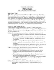
19.4 Utility 

FIGURE 19.6 

Three types of utility 

curves 

Utility 

Dollar Amount 

Panel A: Risk Averter’s Curve 

a. Revise the probabilities of the number of books sold in 

light of the reviewer’s unfavorable review. 



The methods used in Sections 19.1 through 19.3 assume that each incremental amount of profit 

or loss has the same value as the previous amounts of profits attained or losses incurred. In fact, 

under many circumstances in the business world, this assumption of incremental changes is not 

valid. Most companies, as well as most individuals, make special efforts to avoid large losses. At 

the same time, many companies, as well as most individuals, place less value on extremely large 

profits than on initial profits. Such differential evaluation of incremental profits or losses is 

referred to as utility, a concept first discussed by Daniel Bernoulli in the eighteenth century (see 

reference 1). To illustrate this concept, suppose that you are faced with the following two choices: 

Choice 1: A fair coin is to be tossed. If it lands on heads, you will receive $0.60; if it lands 

on tails, you will pay $0.40. 

Choice 2: Do not play the game. 

What decision should you choose? The expected value of playing this game is (0.60)(0.50) + 

(-0.40)(0.50) = +$0.10, and the expected value of not playing the game is 0. 

Most people will decide to play the game because the expected value is positive, and only 

small amounts of money are involved. Suppose, however, that the game is formulated with a 

payoff of $600,000 when the coin lands on heads and a loss of $400,000 when the coin lands on 

tails. The expected value of playing the game is now + $100,000. With these payoffs, even 

though the expected value is positive, most individuals will not play the game because of the 

severe negative consequences of losing $400,000. Each additional dollar amount of either 

profit or loss does not have the same utility as the previous amount. Large negative amounts for 

most individuals have severely negative utility. Conversely, the extra value of each incremental 

dollar of profit decreases when high enough profit levels are reached. (In other words, the difference 

between 0 and $100,000 is much more than the difference between $1,000,000 and 

$1,100,000.) 

An important part of the decision-making process, which is beyond the scope of this text 

(see references 2 and 4), is to develop a utility curve for a decision maker that represents the 

utility of each specified dollar amount. Figure 19.6 illustrates three types of utility curves: 

those of the risk averter, the risk seeker, and the risk-neutral person. 

Utility 

Dollar Amount 

Panel B: Risk Seeker’s Curve 

Utility 

Dollar Amount 

Panel C: Risk-Neutral Curve 

The risk averter’s curve shows a rapid increase in utility for initial amounts of money followed 

by a gradual leveling off for increasing dollar amounts. This curve is appropriate for 

most individuals or businesses because the value of each additional dollar is not as great after 

large amounts of money have already been earned.


Summary 25 

The risk seeker’s curve represents the utility of someone who enjoys taking risks. The 

utility is greater for large dollar amounts. This curve represents an individual who is interested 

only in “striking it rich” and is willing to take large risks for the opportunity of making 

large profits. 

The risk-neutral curve represents the expected monetary value approach. Each additional 

dollar of profit has the same value as the previous dollar. 

After a utility curve is developed in a specific situation, you convert the dollar amounts to 

utilities. Then you compute the utility of each alternative course of action and apply the decision 

criteria of expected utility value, expected opportunity loss, and return-to-risk ratio to 

make a decision. 


19.23 Do you consider yourself a risk seeker, a risk 

averter, or a risk-neutral person? Explain. 

THINK ABOUT THIS Risky Business 

When you make investment decisions, you need 

to think about your own personal tolerance for 

risk. When given the chance to make large sums 

of money, some people can shrug off a 20% 

loss, while others feel ruined when they lose 

even a small amount such as $20. What about 

you? Are you willing to risk losing a lot of money 

for a chance to strike it rich? Or are you more 

comfortable with a less risky scenario, even 

though your chance to strike it rich will be 

smaller? 

How can you identify stocks, mutual funds, 

or other types of investments that fit your own 

personal tolerance for risk? One way to begin is 

to examine the standard deviation of the investments 

you are considering during recent periods 

of time. You will also want to assess your own 

willingness to tolerate different losses. What 

would you do if you lost 10%, 30%, 50%, or 90% 

of your investment? Would you sell? Would you 

buy more in the hope that the investment would 

go back up? Also, think about what you would do 

19.24 Refer to Problems 19.3–19.5 and 19.12–19.14, 

respectively. In which problems do you think the expected 

monetary value (risk-neutral) criterion is inappropriate? 

Why? 

if your investment went up 10%, 50%, 100%, or 

200%. Would you sell the entire investment? Part 

of the investment? Or would you buy more? You 

might want to think about the volatility of your 

investments—that is, any patterns of extreme 

increases and decreases in the value over short 

periods of time—that can add to the risk. 

Everyone is different, but knowing how you 

would answer these questions before you are 

faced with making a decision will help you make 

better investment decisions. 

USING STATISTICS @ The Reliable Fund Revisited 

SUMMARY 

In this chapter, you learned how to develop payoff tables and 

decision trees, to use various criteria to choose between 

In the Using Statistics scenario, you learned how the manager of The 

Reliable Fund could use various decision-making criteria to decide 

whether to purchase stock A or stock B. You also saw how sample 

information could be used to revise probabilities and possibly change 

the decision reached. You found that stock B had a higher expected monetary 

value, a lower expected opportunity loss, but a lower return-to-risk ratio. 

alternative courses of action, and to revise probabilities, 

using Bayes’ theorem, in light of sample information.


KEY EQUATIONS 


N 

EMV(j) = a X ijPi i = 1 

Expected Opportunity Loss 

N 

EOL(j) = a LijPi i = 1 

KEY TERMS 

alternative courses of action 4 

decision criteria 4 

decision tree 4 

events, or states of the world 4 

expected monetary value (EMV) 9 

expected opportunity loss (EOL) 11 

expected profit under certainty 12 

(19.1) 

(19.2) 

expected value of perfect 

information (EVPI) 12 

maximax payoff criterion 8 

maximin payoff criterion 9 

opportunity loss 6 

payoff 4 

payoff table 4 

CHAPTER REVIEW PROBLEMS 

CHECKING YOUR UNDERSTANDING 

19.25 What is the difference between an event and an 

alternative course of action? 

19.26 What are the advantages and disadvantages of a payoff 

table as compared to a decision tree? 

19.27 How are opportunity losses computed from 

payoffs? 

19.28 Why can’t an opportunity loss be negative? 

19.29 How does expected monetary value (EMV) differ 

from expected opportunity loss (EOL)? 

19.30 What is the meaning of the expected value of perfect 

information (EVPI)? 

19.31 How does the expected value of perfect information 

differ from the expected profit under certainty? 

19.32 What are the advantages and disadvantages of using 

expected monetary value (EMV) as compared to the returnto-risk 

ratio (RTRR)? 

19.33 How is Bayes’ theorem used to revise probabilities 

in light of sample information? 

19.34 What is the difference between a risk averter and a 

risk seeker? 

Expected Value of Perfect Information 

EVPI = expected profit under certainty - expected 

monetary value of the best alternative 


RTRR(j) = EMV(j) 

s j 

return-to-risk ratio (RTRR) 14 

risk averter’s curve 24 

risk-neutral curve 25 

risk seeker’s curve 25 

utility 24 

(19.3) 

(19.4) 

19.35 Why should you use utilities instead of payoffs in 

certain circumstances? 


19.36 A supermarket chain purchases large quantities of 

white bread for sale during a week. The stores purchase the 

bread for $0.75 per loaf and sell it for $1.10 per loaf. Any 

loaves not sold by the end of the week can be sold to a local 

thrift shop for $0.40. Based on past demand, the probability 

of various levels of demand is as follows: 

Demand (Loaves) Probability 

6,000 0.10 

8,000 0.50 

10,000 0.30 

12,000 0.10 

a. Construct a payoff table, indicating the events and alternative 



c. Compute the expected monetary value (EMV) for purchasing 

6,000, 8,000, 10,000, and 12,000 loaves. 

d. Compute the expected opportunity loss (EOL) for purchasing 

6,000, 8,000, 10,000, and 12,000 loaves.



f. Based on the results of (c) or (d), how many loaves would 

you purchase? Why? 

g. Compute the coefficient of variation for each purchase 

level. 

h. Compute the return-to-risk ratio (RTRR) for each purchase 

level. 

i. Based on (g) and (h), what action would you choose? 

Why? 

j. Compare the results of (f) and (i) and explain any differences. 

k. Suppose that new information changes the probabilities 

associated with the demand level. Use the following 

probabilities to repeat (c) through (j): 

Demand (Loaves) Probability 

6,000 0.30 

8,000 0.40 

10,000 0.20 

12,000 0.10 

19.37 The owner of a company that supplies home heating 

oil would like to determine whether to offer a solar heating 

installation service to its customers. The owner of the company 

has determined that a startup cost of $150,000 would 

be necessary, but a profit of $2,000 can be made on each 

solar heating system installed. The owner estimates the 

probability of various demand levels as follows: 

Number of Units Installed Probability 

50 0.40 

100 0.30 

200 0.30 

a. Construct a payoff table, indicating the events and alternative 



c. Construct an opportunity loss table. 

d. Compute the expected monetary value (EMV ) for offering 

this solar heating system installation service. 

e. Compute the expected opportunity loss (EOL) for offering 

this solar heating system installation service. 

f. Explain the meaning of the expected value of perfect 


g. Compute the return-to-risk ratio (RTRR) for offering this 

solar heating system installation service. 

h. Based on the results of (d), (e), and (g), should the company 

offer this solar heating system installation service? Why? 

i. How would your answers to (a) through (h) be affected if 

the startup cost were $200,000? 

19.38 The manufacturer of a nationally distributed brand of 

potato chips wants to determine the feasibility of changing 

EVENT 

Chapter Review Problems 27 

the product package from a cellophane bag to an unbreakable 

container. The product manager believes that there are three 

possible national market responses to a change in product 

package: weak, moderate, and strong. The projected payoffs, 

in millions of dollars, in increased or decreased profit compared 

to the current package are as follows: 

Use New 

Package 

STRATEGY 

Keep Old 

Package 

Weak national response -4 0 

Moderate national response 1 0 

Strong national response 5 0 

Based on past experience, the product manager assigns the 

following probabilities to the different levels of national 

response: 

P (Weak national response) = 0.30 

P (Moderate national response) = 0.60 

P (Strong national response) = 0.10 

a. Construct a decision tree. 

b. Construct an opportunity loss table. 

c. Compute the expected monetary value (EMV) for offering 

this new product package. 

d. Compute the expected opportunity loss (EOL) for offering 

this new product package. 



f. Compute the return-to-risk ratio (RTRR) for offering this 

new product package. 

g. Based on the results of (c), (d), and (f), should the company 

offer this new product package? Why? 

h. What are your answers to parts (c) through (g) if the probabilities 

are 0.6, 0.3, and 0.1, respectively? 

i. What are your answers to parts (c) through (g) if the probabilities 

are 0.1, 0.3, and 0.6, respectively? 

Before making a final decision, the product manager would 

like to test market the new package in a selected city by substituting 

the new package for the old package. A determination 

can then be made about whether sales have increased, 

decreased, or stayed the same. In previous test marketing of 

other products, when there was a subsequent weak national 

response, sales in the test city decreased 60% of the time, 

stayed the same 30% of the time, and increased 10% of the 

time. Where there was a moderate national response, sales in 

the test city decreased 20% of the time, stayed the same 40% 

of the time, and increased 40% of the time. When there was 

a strong national response, sales in the test city decreased 

5% of the time, stayed the same 35% of the time, and 

increased 60% of the time. 

j. If sales in the test city stayed the same, revise the original 

probabilities in light of this new information. 

k. Use the revised probabilities in (j) to repeat (c) through (g).


l. If sales in the test city decreased, revise the original 

probabilities in light of this new information. 

m. Use the revised probabilities in (l) to repeat (c) through (g). 

19.39 An entrepreneur wants to determine whether it 

would be profitable to establish a gardening service in a 

local suburb. The entrepreneur believes that there are four 

possible levels of demand for this gardening service: 

Very low demand—1% of the households would use the 

service. 

Low demand—5% of the households would use the service. 

Moderate demand—10% of the households would use 

the service. 

High demand—25% of the households would use the service. 

Based on past experiences in other suburbs, the entrepreneur 

assigns the following probabilities to the various demand levels: 

P(Very low demand) = 0.20 

P(Low demand) = 0.50 

P(Moderate demand) = 0.20 

P(High demand) = 0.10 

The entrepreneur has calculated the following profits or 

losses ($) of this garden service for each demand level (over 

a period of one year): 

DEMAND 

Provide Garden 

Service 

ACTION 

Do Not Provide 

Garden Service 

Very low -50,000 0 

Low 60,000 0 

Moderate 130,000 0 

High 300,000 0 



c. Compute the expected monetary value (EMV ) for offering 

this garden service. 

d. Compute the expected opportunity loss (EOL) for offering 

this garden service. 



f. Compute the return-to-risk ratio (RTRR) for offering this 

garden service. 

g. Based on the results of (c), (d), and (f ), should the entrepreneur 

offer this garden service? Why? 

Before making a final decision, the entrepreneur conducts a 

survey to determine demand for the gardening service. A 

random sample of 20 households is selected, and 3 indicate 

that they would use this gardening service. 

h. Revise the prior probabilities in light of this sample information. 

(Hint: Use the binomial distribution to determine 

the probability of the outcome that occurred, given a particular 

level of demand.) 

i. Use the revised probabilities in (h) to repeat (c) through (g). 

19.40 A manufacturer of a brand of inexpensive felt-tip 

pens maintains a production process that produces 10,000 

pens per day. In order to maintain the highest quality of 

this product, the manufacturer guarantees free replacement 

of any defective pen sold. Each defective pen produced 

costs 20 cents for the manufacturer to replace. Based on 

past experience, four rates of producing defective pens are 

possible: 

Very low—1% of the pens manufactured will be 

defective. 

Low—5% of the pens manufactured will be defective. 

Moderate—10% of the pens manufactured will be 

defective. 

High—20% of the pens manufactured will be defective. 

The manufacturer can reduce the rate of defective pens produced 

by having a mechanic fix the machines at the end of 

each day. This mechanic can reduce the rate to 1%, but his 

services will cost $80. 

A payoff table based on the daily production of 10,000 

pens, indicating the replacement costs ($) for each of the two 

alternatives (calling in the mechanic and not calling in the 

mechanic), is as follows: 

DEFECTIVE RATE 

Do Not Call 

Mechanic 

ACTION 

Call 

Mechanic 

Very low (1%) 20 100 

Low (5%) 100 100 

Moderate (10%) 200 100 

High (20%) 400 100 

Based on past experience, each defective rate is assumed to 

be equally likely to occur. 



c. Compute the expected monetary value (EMV) for calling 

and for not calling the mechanic. 

d. Compute the expected opportunity loss (EOL) for calling 

and for not calling the mechanic. 



f. Compute the return-to-risk ratio (RTRR) for calling and 

not calling the mechanic. 

g. Based on the results of (c), (d), and (f), should the company 

call the mechanic? Why? 

h. At the end of a day’s production, a sample of 15 pens is 

selected, and 2 are defective. Revise the prior probabilities 

in light of this sample information. (Hint: Use the 

binomial distribution to determine the probability of the 

outcome that occurred, given a particular defective 

rate.) 

i. Use the revised probabilities in (h) to repeat (c) 

through (g).

WEB CASE 

Apply your knowledge of decision-making techniques in this 

Web Case, which extends the EndRun Web Case from earlier 

chapters. 

StraightArrow Banking & Investments is a Tri-Cities 

competitor of EndRun that is currently advertising its 

StraightArrow StraightDeal fund. Using a Web browser, 

open to the Web page for the Chapter 19 Web Case (or open 

SA_Home.htm if you have downloaded the Web Case files) 

to visit the StraightArrow Web home page. Examine the 

claims and supporting data for the fund. Compare those 

claims and data to the supporting data found on the EndRun 

Happy Bull and Worried Bear Funds Web page by opening 

to the Web page for the Chapter 5 Web Case (or 

ER_BullsandBears.htm if you have downloaded the Web 

Case files). Then answer the following: 

1. Is the StraightArrow StraightDeal fund a better investment 

than either of the EndRun funds? Support your answer by 

REFERENCES 

1. Bernstein, P. L., Against the Gods: The Remarkable Story 

of Risk (New York: Wiley, 1996). 

2. Microsoft Excel 2007 (Redmond, WA: Microsoft Corp., 

2007). 

3. Render, B., R. M. Stair, and M. Hanna, Quantitative 

Analysis for Management, 9th ed. (Upper Saddle River, 

NJ: Prentice Hall, 2006). 

References 29 

performing an appropriate analysis and summarizing your 

results. 

2. Before making a decision about which fund makes a better 

investment, you decide that you need a reliable forecast 

for the direction of the economy in the next year. 

After further investigation, you find that the consensus of 

leading economists is that the economy will be expanding 

in the next year. You also find out that in the past, when 

there has been a recession, leading economists predicted 

an expanding economy 10% of the time. When there was 

a stable economy, they predicted an expanding economy 

50% of the time, and when there was an expanding economy, 

they predicted an expanding economy 75% of the 

time. When there was a rapidly expanding economy, they 

predicted an expanding economy 90% of the time. Does 

this information change your answer to Question 1? Why 

or why not? 

4. Tversky, A., and D. Kahneman, “Rationale Choice and 

the Framing of Decisions,” Journal of Business, 59 

(1986), 251–278.

CHAPTER 19 EXCEL GUIDE 

EG19.1 PAYOFF TABLES and DECISION 

TREES 

PHStat2 Use the Opportunity Loss procedure to create a 

payoff table and an opportunity loss table. For example, to 

create the payoff and opportunity loss tables for the Example 

19.3 marketing problem on page 6, select PHStat ➔ 

Decision-Making ➔ Opportunity Loss. In the procedure’s 

dialog box (shown below): 

1. Enter 2 as the Number of Events. 

2. Enter 2 as the Number of Alternative Actions. 

3. Enter a Title and click OK. 

In the opportunity loss analysis worksheet that the procedure 

creates, enter the payoff data and event and alternative action 

labels from Table 19.1 in the tinted table cells that begin in row 4. 

(The #DIV/0! messages that may appear in several cells will 

disappear after you enter your data. This is not an error.) 

In-Depth Excel Enter payoff data as a simple table and 

use the INDEX, MATCH, and MAX functions to help 

perform an opportunity loss analysis. Enter INDEX(cell 

range of the alternative action labels, 1,optimum action 

for event) to display the correct alternative course of action 

label. Enter MATCH(cell that contains maximum event 

payoff, cell range of payoffs for event, 0)to determine the 

optimum action for event used by the INDEX function. 

Enter MAX(cell range of payoffs for event) to display the 

optimum profit for an event. 

Use the COMPUTE worksheet of the Opportunity 

Loss workbook, shown in Figure 19.3, as a template for creating 

payoff tables and performing opportunity loss analysis. 

This worksheet performs the analysis for the Example 19.3 

marketing problem that uses the Table 19.1 payoff data on 

page 4. The MATCH function in the column B formulas 

30 

matches the optimum profit found in column C with one of 

two payoff values and returns either the value 1 or 2, 

depending on whether the first or second payoff value 

matched the optimum profit. In turn, INDEX uses the 

returned value (1 or 2) as the column number to decide 

which of the two alternative courses of action labels will be 

displayed in the column B cell. (Open to the COMPUTE_ 

FORMULAS worksheet to examine the details of other formulas 

used in the COMPUTE worksheet.) 

To perform opportunity loss analysis for other problems 

with two events and two alternative courses of action, enter 

the new payoff data and labels in the Payoff Table area in 

rows 4 through 6 in the COMPUTE worksheet. Use the 

COMPUTE_THREE worksheet for problems that contain 

three events and two alternative courses of action, and use 

the COMPUTE_FOUR worksheets for problems that contain 

four events and two alternative courses of action. 

EG19.2 CRITERIA for DECISION MAKING 

PHStat2 Use the Expected Monetary Value procedure to 

create expected monetary value, expected opportunity loss, 

and return-to-risk ratio decision criteria. For example, to 

create the three decision criteria for the Section 19.2 stock 

selection problem, select PHStat ➔ Decision-Making ➔ 

Expected Monetary Value. In the procedure’s dialog box 

(shown below): 

1. Enter 4 as the Number of Events. 

2. Enter 2 as the Number of Alternative Actions. 

3. Check Expected Opportunity Loss. 

4. Check Measures of Variation. 

5. Enter a Title and click OK.

In the worksheet that the procedure creates, enter the probabilities, 

payoff data, and event and alternative action labels from 

Table 19.10 in the tinted table cells that begin in row 4. (The 

#DIV/0! messages that may appear in several cells will disappear 

after you enter your data. This is not an error.) 

In-Depth Excel Use the SUMPRODUCT function to 

compute the expected monetary value and variance and use 

the INDEX, MATCH, and MAX functions (discussed in the 

Section EG19.1 In-Depth Excel instructions) to help perform 

an opportunity loss analysis. Enter SUMPRODUCT(cell 

range of the probabilities of the events, cell range of the 

payoffs for one alternative course of action) to compute the 

expected monetary value and enter SUMPRODUCT(cell 

range of the probabilities of the events, cell range of 

Chapter 19 Excel Guide 31 

squared differences for one alternative course of action) to 

compute the variance. 

Use the COMPUTE worksheet of the Expected 

Monetary Value workbook, shown in Figure 19.4, as a template 

for creating expected monetary value, expected opportunity 

loss, and the return-to-risk ratio decision criteria. This 

worksheet creates the decision criteria for the Section 19.2 

stock selection problem. Open to the COMPUTE_ 

FORMULAS worksheet to examine the details of all formulas 

used in the COMPUTE worksheet. 

To create decision criteria for other problems involving 

four events and two alternative courses of action, make new 

entries in the Probabilities & Payoff Table area. Use the 

COMPUTE_THREE worksheet for problems that contain 

three events and two alternative courses of action.

19.1 Payoff Tables and Decision Trees

You also want an ePaper? Increase the reach of your titles

Delete template?

Save as template?