BMJ Statistical Notes Series List by JM Bland: http://www-users.york ...

More documents

Recommendations

Info

distinguish between psychiatric patients and medical patients? Do we get different anxiety scores from students before and after an examination? Does a measure of depression predict suicide attempts? We call the property of having appropriate relationships with other variables construct validity. We can also ask whether the items which together compose the scale are related to one another: does the scale have internal consistency? If not, do the items really measure the same thing? On the other hand, if the items are too similar, some may be redundant. Highly correlated items in a scale may make the scale overlong and may lead to some aspects being overemphasised, impairing the content validity. A handy summary measure for this feature is Cronbach’s alpha. 5 A scale must also be repeatable and be sufficiently objective to give similar results for different observers. If a measurement is repeatable, in that someone who has a high score on one occasion tends to have a high score on another, it must be measuring something. With physical measurements, it is often possible for the same observer (or different observers) to make repeated measurements in quick succession. When there is a subjective element in the measurement the observer can be blinded from their first measurement, Honour a physician with the honour due unto him A few years ago my general practitioner told me that anyone aged over 40 with upper abdominal discomfort needed investigating. At the local teaching hospital, a pleasant young doctor did a gastroscopy, which showed a mass in my stomach wall. I was sent for a barium meal. A consultant radiologist took the x ray films, instructing me briskly to turn this way and that but not otherwise paying me any attention. He told me to wait a few minutes while he checked the films to see if all the views were satisfactory. I sat alone in the room for about five minutes. From the moment the consultant re-entered I could see that he was slightly agitated. “I’m terribly sorry,” he called out as he came through the door at the far end. And then again, “I’m terribly sorry.” Perhaps these words of regret, coupled with the concern on his face, might not have had the effect they did had I not been a man with an abdominal mass on his mind. At this moment of truth and reckoning, certain visions swam before my eyes. Three strides later, he was in front of me and looking me full in the face: “I’m terribly sorry, I hadn’t realised you were a doctor.” In his hand was the request form, and I could see that my general practitioner had written “ex-SR here” in one corner. He must have spotted this when checking the form as he looked at the preliminary plates. Though no further x rays were needed, he proceeded a little breathlessly to deliver three or four minutes of almost a caricature of caring, empathic interest in a patient. What branch of medicine was I in, and where did I work? Good heavens, that must be tough. Is that an Australian accent I hear? A St Mary’s old boy, ah yes. What did I think about. . .? I don’t mean to imply that this was insincere, merely splendidly different from his earlier matter of factness and economy of word. I had thought nothing of this at the time: in such a bread and butter procedure I had BMJ VOLUME 324 9 MARCH 2002 bmj.com Downloaded from bmj.com on 28 February 2008 and different observers can make simultaneous measurements. In assessing the reliability of a website quality scale, it is easy to get several observers to apply the scale independently. With websites, repeat assessments need to be close in time because their content changes frequently (as does bmj.com). With questionnaires, either self administered or recorded by an observer, repeat measurements need to be far enough apart in time for the earlier responses to be forgotten, yet not so far apart that the underlying quantity being measured might have changed. Such data enable us to evaluate test-retest reliability. If two measures have comparable face, content, and construct validity the more repeatable one may be preferred for the study of a given population. 1 Gagliardi A, Jadad AR. Examination of instruments used to rate quality of health information on the internet: chronicle of a voyage with an unclear destination. BMJ 2002;324:569-73. 2 Jüni P, Altman DG, Egger M. Assessing the quality of controlled clinical trials. BMJ 2001;323:42-6. 3 Muldoon MF, Barger SD, Flory JD, Manuck B. What are quality of life measurements measuring? BMJ 1998;316:542-5. 4 Streiner DL, Norman GR. Health measurement scales: a practical guide to their development and use. 2nd ed. Oxford: Oxford University Press, 1996. 5 Bland JM, Altman DG. Cronbach’s alpha. BMJ 1997;314:572. no more reason to expect the doctor to engage with me as a person than I would the phlebotomist taking a routine blood sample. Clearly, this consultant saw things similarly as a rule, but when the patient was a doctor the aesthetics of the encounter changed. He had apologised three times for what he felt was a lapse on his part, arising from his failure to notice what was written in the corner of the request form. Perhaps he thought I knew that my general practitioner had written this and that I expected this of a medical referral, and thus expected to be recognised by him not just as a patient but also as a colleague. He seemed to see this as my due. (As it happens, I didn’t.) I had forgotten this incident, but it was brought back to me by the aftermath of the Bristol cardiac surgery debacle, and by the publicity surrounding other recent medical scandals. These have all put a spotlight on relations between doctors, who seem to offer each other acknowledgement and empathy, as my consultant had sought belatedly to do to me. The general public may be coming to suspect that this collegiate solidarity is somehow not in their interests, associating it with mutual protectiveness and thus with cover-ups of medical malpractice. It is too soon to say how the profession will react, but my consultant was an older man and my guess is that, with younger generations of doctors, we will see the waning of a tradition whose roots lie with Hippocrates. For it was his oath that bound doctors to look well on each other (and not charge each other for their services). It’s another story, but I found out later that the mass was the gastroscopy instrument itself distorting the stomach wall, misdiagnosed by an inexperienced registrar. No special treatment there, anyway. Derek Summerfield consultant psychiatrist, CASCAID, South London and Maudsley NHS Trust, London Education and debate 607
Statistics Notes Interaction revisited: the difference between two estimates Douglas G Altman, J Martin Bland We often want to compare two estimates of the same quantity derived from separate analyses. Thus we might want to compare the treatment effect in subgroups in a randomised trial, such as two age groups. The term for such a comparison is a test of interaction. In earlier Statistics Notes we discussed interaction in terms of heterogeneity of treatment effect. 1–3 Here we revisit interaction and consider the concept more generally. The comparison of two estimated quantities, such as means or proportions, each with its standard error, is a general method that can be applied widely. The two estimates should be independent, not obtained from the same individuals—examples are the results from subgroups in a randomised trial or from two independent studies. The samples should be large. If the estimates are E 1 and E 2 with standard errors SE(E 1) and SE(E 2), then the difference d=E 1 − E 2 has standard error SE(d)=√[SE(E 1) 2 + SE(E 2) 2 ] (that is, the square root of the sum of the squares of the separate standard errors). This formula is an example of a well known relation that the variance of the difference between two estimates is the sum of the separate variances (here the variance is the square of the standard error). Then the ratio z=d/SE(d) gives a test of the null hypothesis that in the population the difference d is zero, by comparing the value of z to the standard normal distribution. The 95% confidence interval for the difference is d−1.96SE(d) tod+1.96SE(d). We illustrated this for means and proportions, 3 although we did not show how to get the standard error of the difference. Here we consider comparing relative risks or odds ratios. These measures are always analysed on the log scale because the distributions of the log ratios tend to be those closer to normal than of the ratios themselves. In a meta-analysis of non-vertebral fractures in randomised trials of hormone replacement therapy the estimated relative risk from 22 trials was 0.73 (P=0.02) in favour of hormone replacement therapy. 4 From 14 trials of women aged on average < 60 years the relative risk was 0.67 (95% confidence interval 0.46 to 0.98; P=0.03). From eight trials of women aged >60 the relative risk was 0.88 (0.71 to 1.08; P=0.22). In other words, in younger women the estimated treatment benefit was a 33% reduction in risk of fracture, which was statistically significant, compared with a 12% reduction in older women, which was not significant. But are the relative risks from the subgroups significantly different from each other? We show how to answer this question using just the summary data quoted. 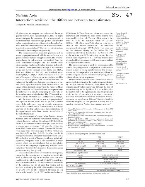Because the calculations were made on the log scale, comparing the two estimates is complex (see table). We need to obtain the logs of the relative risks and their confidence intervals (rows 2 and 4). 5 As 95% confidence intervals are obtained as 1.96 standard errors either side of the estimate, the SE of each log relative risk is obtained by dividing the width of its confidence interval by 2×1.96 (row 6). The estimated difference in log relative risks is d=E 1− E 2=−0.2726 and its standard error BMJ VOLUME 326 25 JANUARY 2003 bmj.com Downloaded from bmj.com on 28 February 2008 0.2206 (row 8). From these two values we can test the interaction and estimate the ratio of the relative risks (with confidence interval). The test of interaction is the ratio of d to its standard error: z=−0.2726/ 0.2206=−1.24, which gives P=0.2 when we refer it to a table of the normal distribution. The estimated interaction effect is exp( − 0.2726)=0.76. (This value can also be obtained directly as 0.67/0.88=0.76.) The confidence interval for this effect is − 0.7050 to 0.1598 on the log scale (row 9). Transforming back to the relative risk scale, we get 0.49 to 1.17 (row 12). There is thus no good evidence to support a different treatment effect in younger and older women. The same approach is used for comparing odds ratios. Comparing means or regression coefficients is simpler as there is no log transformation. The two estimates must be independent: the method should not be used to compare a subset with the whole group, or two estimates from the same patients. There is limited power to detect interactions, even in a meta-analysis combining the results from several studies. As this example illustrates, even when the two estimates and P values seem very different the test of interaction may not be significant. It is not sufficient for the relative risk to be significant in one subgroup and not in another. Conversely, it is not correct to assume that when two confidence intervals overlap the two estimates are not significantly different. 6 Statistical analysis should be targeted on the question in hand, and not based on comparing P values from separate analyses. 2 1 Altman DG, Matthews JNS. Interaction 1: Heterogeneity of effects. BMJ 1996;313:486. 2 Matthews JNS, Altman DG. Interaction 2: Compare effect sizes not P values. BMJ 1996;313:808. 3 Matthews JNS, Altman DG. Interaction 3: How to examine heterogeneity. BMJ 1996;313:862. 4 Torgerson DJ, Bell-Syer SEM. Hormone replacement therapy and prevention of nonvertebral fractures. A meta-analysis of randomized trials. JAMA 2001;285:2891-7. 5 Bland JM, Altman DG. Logarithms. BMJ 1996;312:700. 6 Bland M, Peacock J. Interpreting statistics with confidence. Obstetrician and Gynaecologist (in press). Calculations for comparing two estimated relative risks Education and debate Cancer Research UK Medical Statistics Group, Centre for Statistics in Medicine, Institute for Health Sciences, Oxford OX3 7LF Douglas G Altman professor of statistics in medicine Department of Public Health Sciences, St George’s Hospital Medical School, London SW17 0RE J Martin Bland professor of medical statistics Correspondence to: D G Altman doug.altman@ cancer.org.uk BMJ 2003;326:219 Group 1 Group 2 1 RR 0.67 0.88 2 *log RR −0.4005 (E1) −0.1278 (E2) 3 95% CI for RR 0.46 to 0.98 0.71 to 1.08 4 *95% CI for log RR −0.7765 to −0.0202 −0.3425 to 0.0770 5 Width of CI 0.7563 0.4195 6 SE[=width/(2×1.96)] 0.1929 0.1070 Difference between log relative risks 7 d[=E1−E2] −0.4005–(−0.1278)=−0.2726 8 SE(d) √(0.1929 2 + 0.1070 2 )=0.2206 9 CI(d) −0.2726 ±1.96×0.2206 or −0.7050 to 0.1598 10 Test of interaction z=−0.2726/0.2206=−1.24 (P=0.2) Ratio of relative risks (RRR) 11 RRR=exp(d) exp(−0.2726)=0.76 12 CI(RRR) exp(−0.7050) to exp(0.1598), or 0.49 to 1.17 *Values obtained by taking natural logarithms of values on preceding row. 219
Page 1 and 2:
BMJ Statistical Notes Series List b
Page 3 and 4:
BMJ Statistical Notes Series List b
Page 5 and 6:
Downloaded from bmj.com on 28 Febru
Page 7 and 8: Downloaded from bmj.com on 28 Febru
Page 25 and 26: i . ~~ " . It ~, I ; Statistics Not
Page 27 and 28: .'.)'. In practice, there will usua
Page 45 and 46: Statistics notes Bayesians and freq
Page 47 and 48: Statistics notes Treatment allocati
Page 49 and 50: Much work still needs to be done to
Page 51 and 52: Education and debate Department of
Page 53 and 54: Education and debate ICRF Medical S
Page 55 and 56: Statistics Notes Analysing controll
Page 57: Education and debate Papers p569 De
Page 61 and 62: Papers What is already known on thi
Page 63 and 64: test results. Forcing dichotomisati
Page 65 and 66: 6 The Cardiac Arrhythmia Suppressio
Page 67 and 68: PRACTICE 1 Cancer Research UK/NHS C
Page 69 and 70: 1 Department of Health Sciences, Un
Page 71 and 72: BMJ 2011;342:d561 doi: 10.1136/bmj.
Page 73 and 74: BMJ 2011;342:d561 doi: 10.1136/bmj.
Page 75 and 76: RESEARCH METHODS AND REPORTING, p 6
Page 77: RESEARCH METHODS & REPORTING 1 Cent
show all

BMJ Statistical Notes Series List by JM Bland: http://www-users.york ...

You also want an ePaper? Increase the reach of your titles

Delete template?

Save as template?