On the Identification of Misspecified Propensity Scores - School of ...

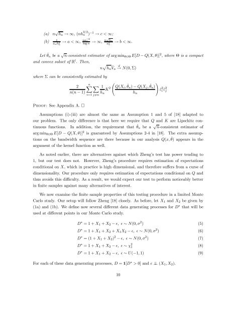
(a) n √ hn → ∞, (nh 3/2
n ) −1 → c < ∞;
(b)
1
anh 2 n
→ a < ∞, na−2 n
log n → ∞, n√hn a2 n
→ b < ∞.
Let ˆ θn be a √ n-consistent estimator of arg minθ∈Θ E[D − Q(X, θ)] 2 , where Θ is a compact
and convex subset of R l . Then,
hn
i=1 j=n
n hn ˆVn d → N(0, Σ)
where Σ can be consistently estimated by
n 2
n(n − 1)
1
K 2
Q(Xi, ˆ θn) − Q(Xj, ˆ
θn)
P: See Appendix A.
Assumptions (i)-(iii) are almost the same as Assumption 1 and 5 of [18] adapted to
our problem. The only difference is that here we require that Q and K are Lipschitz con-
tinuous functions. In addition, the requirement that ˆ θn be a √ n-consistent estimator of
arg minθ∈Θ E[D − Q(X, θ)] 2 is guaranteed by Assumptions 2-4 in [18]. The extra assump-
tions on the bandwidth sequence are there because in our analysis Q(x, ˆ θ) appears in the
argument of the kernel function as well.
As noted earlier, there are alternatives against which Zheng’s test has power tending to
1, but our test does not. However, Zheng’s procedure requires estimation of expectations
conditional on X, which in practice is high dimensional, and therefore suffers from a curse of
dimensionality. Our procedure only requires estimation of expectations conditional on Q and
thus avoids this difficulty. As a result, we would expect our test to perform noticeably better
in finite samples against many alternatives of interest.
We now examine the finite sample properties of this testing procedure in a limited Monte
Carlo study. Our setup will follow Zheng [18] closely. As before, let X1 and X2 be given by
(1a) and (1b). We define now several different data generating processes for D ∗ that will be
used at different points in our Monte Carlo study.
hn
ˆε 2 i ˆε 2 j
D ∗ = 1 + X1 + X2 − ǫ, ǫ ∼ N(0, σ 2 ) (5)
D ∗ = 1 + X1 + X2 + X1X2 − ǫ, ǫ ∼ N(0, σ 2 ) (6)
D ∗ = (1 + X1 + X2) 2 − ǫ, ǫ ∼ N(0, σ 2 ) (7)
D ∗ = 1 + X1 + X2 − ǫ, ǫ ∼ χ 2 1
D ∗ = 1 + X1 + X2 − ǫ, ǫ ∼ U(−1, 1) (9)
For each of these data generating processes, D = 1[D ∗ > 0] and ǫ ⊥ (X1, X2).
10
(8)