On the Identification of Misspecified Propensity Scores - School of ...

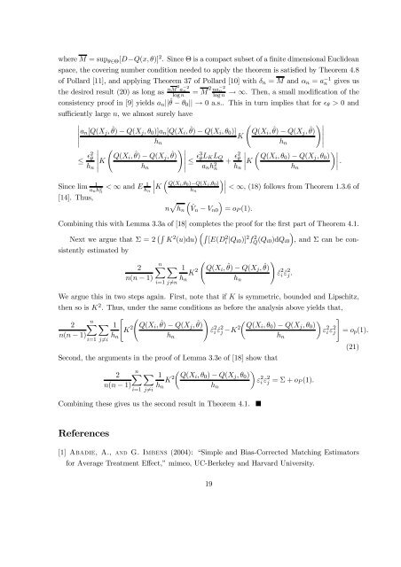
where M = sup θ∈Θ[D−Q(x, θ)] 2 . Since Θ is a compact subset of a finite dimensional Euclidean
space, the covering number condition needed to apply the theorem is satisfied by Theorem 4.8
of Pollard [11], and applying Theorem 37 of Pollard [10] with δn = M and αn = a −1
n
the desired result (20) as long as nM2a −2
n
log n
= M 2 na −2
n
log n
gives us
→ ∞. Then, a small modification of the
consistency proof in [9] yields an|| ˆ θ − θ0|| → 0 a.s.. This in turn implies that for ǫθ > 0 and
sufficiently large n, we almost surely have
an[Q(Xj,
ˆ θ) − Q(Xj, θ0)]an[Q(Xi, ˆ
θ) − Q(Xi, θ0)] Q(Xi,
K
hn
ˆ θ) − Q(Xj, ˆ
θ)
hn
K
Q(Xi, ˆ θ) − Q(Xj, ˆ
θ)
≤ ǫ3 θLKLQ
K
Q(Xi, θ0) − Q(Xj, θ0)
.
≤ ǫ2 θ
hn
Since lim 1
anh 2 n
[14]. Thus,
hn
< ∞ and E 1
K hn
anh 2 n
Q(Xi,θ0)−Q(Xj,θ0)
hn
+ ǫ2 θ
hn
n
hn
ˆVn − Vn0 = oP (1).
hn
< ∞, (18) follows from Theorem 1.3.6 of
Combining this with Lemma 3.3a of [18] completes the proof for the first part of Theorem 4.1.
Next we argue that Σ = 2 K2 (u)du [E(D2 i |Qi0)] 2f 2 Q (Qi0)dQi0
, and Σ can be consistently
estimated by
n 2 1
K
n(n − 1)
2
Q(Xi, ˆ θ) − Q(Xj, ˆ
θ)
ˆε 2 i ˆε 2 j.
hn
i=1 j=n
We argue this in two steps again. First, note that if K is symmetric, bounded and Lipschitz,
then so is K2 . Thus, under the same conditions as before the analysis above yields that,
n
2 1
K
n(n − 1)
2
Q(Xi, ˆ θ) − Q(Xj, ˆ
θ)
ˆε 2 i ˆε 2 j −K 2
Q(Xi, θ0) − Q(Xj, θ0)
ε 2 i ε 2
j = op(1).
hn
i=1 j=i
hn
Second, the arguments in the proof of Lemma 3.3e of [18] show that
hn
i=1 j=i
hn
n 2 1
K
n(n − 1)
2
Q(Xi, θ0) − Q(Xj, θ0)
Combining these gives us the second result in Theorem 4.1.
References
hn
hn
ε 2 i ε 2 j = Σ + oP (1).
[1] A, A., G. I (2004): “Simple and Bias-Corrected Matching Estimators
for Average Treatment Effect,” mimeo, UC-Berkeley and Harvard University.
19
(21)