Solitons in Nonlocal Media

2.5 Theory of Nonlinear Optical Propagation in NLC
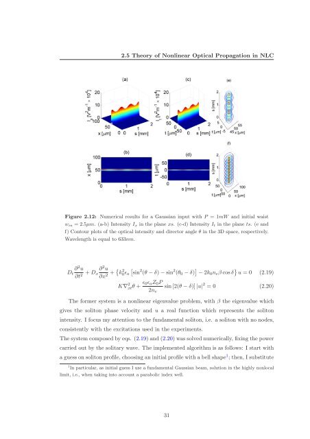
Figure 2.12: Numerical results for a Gaussian input with P = 1mW and initial waist
win = 2.5µm. (a-b) Intensity Ix in the plane xs. (c-d) Intensity It in the plane ts. (e and
f) Contour plots of the optical intensity and director angle θ in the 3D space, respectively.
Wavelength is equal to 633nm.
Dt
∂ 2 u
∂t
2 + Dx
∂2u ∂x2 + k 2 2 2
0ǫa sin (θ − δ) − sin (θ0 − δ) − 2k0neβ cos δ u = 0 (2.19)
K∇ 2 xtθ + ǫ0ǫaZ0P
2ne
sin[2(θ − δ)] |u| 2 = 0 (2.20)
The former system is a nonlinear eigenvalue problem, with β the eigenvalue which
gives the soliton phase velocity and u a real function which represents the soliton
intensity. I focus my attention to the fundamental soliton, i.e. a soliton with no nodes,
consistently with the excitations used in the experiments.
The system composed by eqs. (2.19) and (2.20) was solved numerically, fixing the power
carried out by the solitary wave. The implemented algorithm is as follows: I start with
a guess on soliton profile, choosing an initial profile with a bell shape 1 ; then, I substitute
1 In particular, as initial guess I use a fundamental Gaussian beam, solution in the highly nonlocal
limit, i.e., when taking into account a parabolic index well.
31