Solitons in Nonlocal Media

3.4 Soliton Oscillations in a Finite-Size Geometry
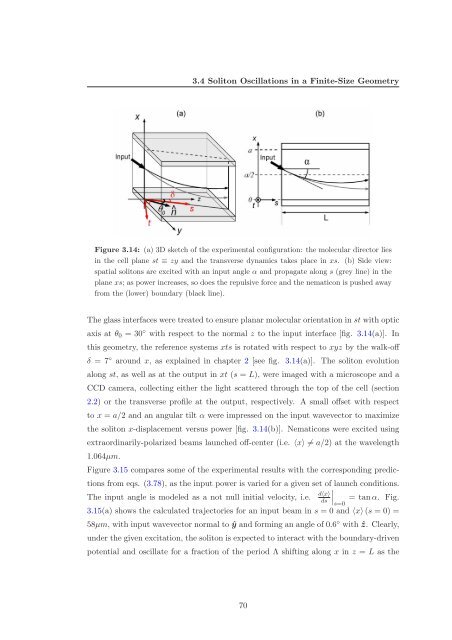
Figure 3.14: (a) 3D sketch of the experimental configuration: the molecular director lies
in the cell plane st ≡ zy and the transverse dynamics takes place in xs. (b) Side view:
spatial solitons are excited with an input angle α and propagate along s (grey line) in the
plane xs; as power increases, so does the repulsive force and the nematicon is pushed away
from the (lower) boundary (black line).
The glass interfaces were treated to ensure planar molecular orientation in st with optic
axis at θ0 = 30 ◦ with respect to the normal z to the input interface [fig. 3.14(a)]. In
this geometry, the reference systems xts is rotated with respect to xyz by the walk-off
δ = 7 ◦ around x, as explained in chapter 2 [see fig. 3.14(a)]. The soliton evolution
along st, as well as at the output in xt (s = L), were imaged with a microscope and a
CCD camera, collecting either the light scattered through the top of the cell (section
2.2) or the transverse profile at the output, respectively. A small offset with respect
to x = a/2 and an angular tilt α were impressed on the input wavevector to maximize
the soliton x-displacement versus power [fig. 3.14(b)]. Nematicons were excited using
extraordinarily-polarized beams launched off-center (i.e. 〈x〉 = a/2) at the wavelength
1.064µm.
Figure 3.15 compares some of the experimental results with the corresponding predic-
tions from eqs. (3.78), as the input power is varied for a given set of
launch conditions.
The input angle is modeled as a not null initial velocity, i.e. = tanα. Fig.
s=0
3.15(a) shows the calculated trajectories for an input beam in s = 0 and 〈x〉 (s = 0) =
58µm, with input wavevector normal to ˆy and forming an angle of 0.6 ◦ with ˆz. Clearly,
under the given excitation, the soliton is expected to interact with the boundary-driven
potential and oscillate for a fraction of the period Λ shifting along x in z = L as the
70
d〈x〉
ds