WOC 6e Guide to Microscopy

Principles and Techniques
of Microscopy
Cell biologists often need to examine the structure of cells
and their components. The microscope is an indispensable
tool for this purpose because most cellular structures are
too small to be seen by the unaided eye. In fact, the beginnings
of cell biology can be traced to the invention of the
light microscope, which made it possible for scientists to see
enlarged images of cells for the first time. The first generally
useful light microscope was developed in 1590 by Z. Janssen
and his nephew H. Janssen. Many important microscopic observations
were reported during the next century, notably
those of Robert Hooke, who observed the first cells, and
Antonie van Leeuwenhoek, whose improved microscopes
provided our first glimpses of internal cell structure. Since
then, the light microscope has undergone numerous improvements
and modifications, right up to the present time.
Just as the invention of the light microscope heralded a
wave of scientific achievement by allowing us to see cells for
the first time, the development of the electron microscope in
the 1930s revolutionized our ability to explore cell structure
and function. Because it is at least a hundred times better at
visualizing objects than the light microscope, the electron
microscope ushered in a new era in cell biology, opening our
eyes to an exquisite subcellular architecture never before seen
and changing forever the way we think about cells.
But in spite of its inferior resolving power, the light
microscope has not fallen into disuse. To the contrary, light
microscopy has experienced a renaissance in recent years as
the development of specialized new techniques has allowed
researchers to explore aspects of cell structure and behavior
that cannot be readily studied by electron microscopy. These
advances have involved the merging of technologies from
physics, engineering, chemistry, and molecular biology, and
they have greatly expanded our ability to study cells using the
light microscope.
In this Appendix, we will explore the fundamental principles
of both light and electron microscopy, placing emphasis
on the various specialized techniques that are used to
adapt these two types of microscopy for a variety of specialized
purposes.
Optical Principles of Microscopy
Appendix
Although light and electron microscopes differ in many
ways, they make use of similar optical principles to form
images. Therefore, we begin our discussion of microscopy by
examining these underlying common principles, placing special
emphasis on the factors that determine how small an
object it is possible to see.
THE ILLUMINATING WAVELENGTH SETS A LIMIT
ON HOW SMALL AN OBJECT CAN BE SEEN
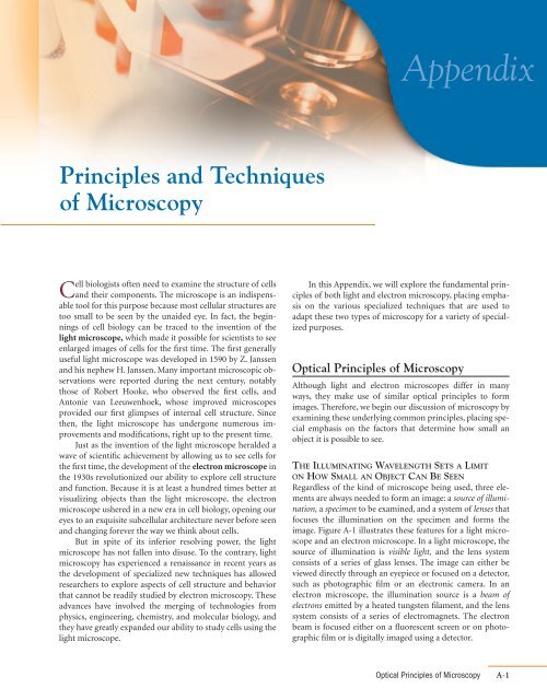
Regardless of the kind of microscope being used, three elements
are always needed to form an image: a source of illumination,
a specimen to be examined, and a system of lenses that
focuses the illumination on the specimen and forms the
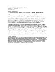
image. Figure A-1 illustrates these features for a light microscope
and an electron microscope. In a light microscope, the
source of illumination is visible light, and the lens system
consists of a series of glass lenses. The image can either be
viewed directly through an eyepiece or focused on a detector,
such as photographic film or an electronic camera. In an
electron microscope, the illumination source is a beam of
electrons emitted by a heated tungsten filament, and the lens
system consists of a series of electromagnets. The electron
beam is focused either on a fluorescent screen or on photographic
film or is digitally imaged using a detector.
Optical Principles of Microscopy A-1

Visible light
Light source
Glass lenses Electromagnetic lenses
Human eye, photographic
film, or electronic detector
(video camera)
Condenser lenses
Specimens
Objective lenses
Intermediate lenses
Ocular lens
50–100 kV
Projector lens
Fluorescent viewing screen
or photographic film
A-2 Appendix Principles and Techniques of Microscopy
Tungsten filament
Beam of electrons
Anode
(a) The light microscope (b) The electron microscope
Despite these differences in illumination source and
instrument design, both types of microscopes depend on the
same principles of optics and form images in a similar manner.
When a specimen is placed in the path of a light or electron
beam, physical characteristics of the beam are changed
in a way that creates an image that can be interpreted by the
human eye or recorded on a photographic detector. To
understand this interaction between the illumination source
and the specimen, we need to understand the concept of
wavelength, which is illustrated in Figure A-2 using the following
simple analogy.
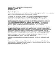
If two people hold onto opposite ends of a slack rope
and wave the rope with a rhythmic up-and-down motion,
they will generate a long, regular pattern of movement in
the rope called a wave form (Figure A-2a). The distance from
the crest of one wave to the crest of the next is called the
wavelength. If someone standing to one side of the rope
tosses a large object such as a beach ball toward the rope, the
ball may interfere with, or perturb, the wave form of the
rope’s motion (Figure A-2b). However, if a small object such
as a softball is tossed toward the rope, the movement of the
rope will probably not be affected at all (Figure A-2c). If
the rope holders move the rope more rapidly, the motion of
the rope will still have a wave form, but the wavelength will
be shorter (Figure A-2d). In this case, a softball tossed toward
−
+
Figure A-1 The Optical Systems of the Light
Microscope and the Electron Microscope.
(a) The light microscope uses visible light
and glass lenses to form an image of the
specimen that can be seen by the eye,
focused on photographic film, or received by
an electronic detector such as a video camera.
(b) The electron microscope uses a
beam of electrons emitted by a tungsten filament
and focused by electromagnetic lenses
to form an image of the specimen on a fluorescent
screen, a digital detector, or photographic
film. (These diagrams have been
drawn to emphasize the similarities in overall
design between the two types of microscope.
In reality, a light microscope is
designed with the light source at the bottom
and the ocular lens at the top, as shown in
Figure 5b.)
the rope is quite likely to perturb the rope’s movement
(Figure A-2e).
This simple analogy illustrates an important principle:
The ability of an object to perturb a wave motion depends
crucially on the size of the object in relation to the wavelength
of the motion. This principle is of great importance in
microscopy, because it means that the wavelength of the illumination
source sets a limit on how small an object can be
seen. To understand this relationship, we need to recognize
that the moving rope of Figure A-2 is analogous to the beam
of light (photons) or electrons that is used as an illumination
source in a light or electron microscope, respectively—in
other words, both light and electrons behave as waves. When
a beam of light or electrons encounters a specimen, the specimen
alters the physical characteristics of the illuminating
beam, just as the beach ball or softball alters the motion of
the rope. And because an object can be detected only by its
effect on the wave, the wavelength must be comparable in
size to the object that is to be detected.
Once we understand this relationship between wavelength
and object size, we can readily appreciate why very
small objects can be seen only by electron microscopy: The
wavelengths of electrons are very much shorter than those of
photons. Thus, objects such as viruses and ribosomes are too
small to perturb a wave of photons, but they can readily

(a)
(b)
(c)
(d)
(e)
Wave form
Wavelength
Wavelength
Softball
Beach ball
Figure A-2 Wave Motion, Wavelength, and Perturbations. The
wave motion of a rope held between two people is analogous to the
wave form of both photons and electrons, and can be used to illustrate
the effect of the size of an object on its ability to perturb wave
motion. (a) Moving a slack rope up and down rhythmically will
generate a wave form with a characteristic wavelength. (b) When
thrown against a rope, a beach ball, or other object with a diameter
that is comparable to the wavelength of the rope will perturb the
motion of the rope. (c) A softball or other object with a diameter
significantly less than the wavelength of the rope will cause little or
no perturbation of the rope. (d) If the rope is moved more rapidly,
the wavelength will be reduced substantially. (e) A softball can now
perturb the motion of the rope because its diameter is comparable
to the wavelength of the rope.
interact with a wave of electrons. As we discuss different
types of microscopes and specimen preparation techniques,
you might find it helpful to ask yourself how the source and
specimen are interacting and how the characteristics of both
are modified to produce an image.
RESOLUTION REFERS TO THE ABILITY
TO DISTINGUISH ADJACENT OBJECTS
AS SEPARATE FROM ONE ANOTHER
When waves of light or electrons pass through a lens and
come to a focus, the image that is formed results from a property
of waves called interference—the process by which two
or more waves combine to reinforce or cancel one another,
producing a wave equal to the sum of the two combining
waves. Thus, the image that you see when you look at a specimen
through a series of lenses is really just a pattern of either
additive or canceling interference of the waves that went
through the lenses, a phenomenon known as diffraction.
In a light microscope, glass lenses are used to direct the
course of photons, whereas an electron microscope uses electromagnets
as lenses to direct the course of electrons. Yet
both kinds of lenses have two fundamental properties in
common: focal length and angular aperture. The focal length
is the distance between the midline of the lens and the point
at which rays passing through the lens converge to a focus
(Figure A-3). The angular aperture is the half-angle a
of the
cone of light entering the objective lens of the microscope
from the specimen (Figure A-4). Angular aperture is therefore
a measure of how much of the illumination that leaves
the specimen actually passes through the lens. This in turn
determines the sharpness of the interference pattern,
and therefore the ability of the lens to convey information
about the specimen. In the best light microscopes, the angular
aperture is about 70 ° .
The angular aperture of a lens is one of the factors that
influences a microscope’s resolution, which is defined as the
minimum distance that can separate two points that still
remain identifiable as separate points when viewed through
the microscope.
Parallel rays
Midline
of lens
Focal length
Focal
point
Figure A-3 The Focal Length of a Lens. Focal length is the distance
from the midline of a lens to the point at which parallel rays
passing through the lens converge to a focus.
Optical Principles of Microscopy A-3

Objective lens
Specimen Image
Objective lens
(a) Low-aperture lens (b) High-aperture lens
Figure A-4 The Angular Aperture of a Lens. The angular aperture
is the half-angle a of the cone of light entering the objective lens of
the microscope from the specimen. (a) A low-aperture lens ( a is
small). (b) A high-aperture lens ( a is large). The larger the angular
aperture, the more information the lens can transmit. The best
glass lenses have an angular aperture of about 70°.
A-4 Appendix Principles and Techniques of Microscopy
Specimen Image
Resolution is governed by three factors: the wavelength
of the light used to illuminate the specimen, the angular
aperture, and the refractive index of the medium surrounding
the specimen. (Refractive index is a measure of the
change in the velocity of light as it passes from one medium
to another.) The effect of these three variables on resolution
is described quantitatively by the following equation known
as the Abbé equation:
r= (A-1)
where r is the resolution, l is the wavelength of the light used
for illumination, n is the refractive index of the medium
between the specimen and the objective lens of the microscope,
and a is the angular aperture as already defined. The constant
0.61 represents the degree to which image points can overlap
and still be recognized as separate points by an observer.
In the preceding equation, the quantity n sin a is called
the numerical aperture of the objective lens, abbreviated
NA. An alternative expression for resolution is therefore
0.61l
n sin a ,
r= 0.61l
NA .
(A-2)
THE PRACTICAL LIMIT OF RESOLUTION IS ROUGHLY
200 NM FOR LIGHT MICROSCOPY AND 2 NM FOR
ELECTRON MICROSCOPY
Maximizing resolution is an important goal in both light and
electron microscopy. Because r is a measure of how close two
points can be and still be distinguished from each other, resolution
improves as r becomes smaller. Thus, for the best resolution,
the numerator of equation A-2 should be as small as
possible and the denominator should be as large as possible.
We will begin by asking how to maximize resolution for
a glass lens with visible light as the illumination source. First,
we need to make the numerator as small as possible. The
wavelength for visible light falls in the range of 400–700 nm,
so the minimum value for l
is set by the shortest wavelength
in this range that is practical to use for illumination, which
turns out to be blue light of about 450 nm. To maximize the
denominator of equation A-2, recall that the numerical aperture
is the product of the refractive index and the sine of the
angular aperture. Both of these values must therefore be
maximized to achieve optimal resolution. Since the angular
aperture for the best objective lenses is about 70 ° , the maximum
value for sin a is about 0.94. The refractive index of air
is about 1.0, so for a lens designed for use in air, the maximum
numerical aperture is about 0.94.
Thus, for a lens with an angular aperture of 70°, the resolution
in air for a sample illuminated with blue light of 450
nm can be calculated as follows:
=
(0.61)(450)
r=
=292 nm.
0.94
0.61l
NA
(A-3)
As a rule of thumb, then, the limit of resolution for a glass
lens in air is roughly 300 nm.
As a means of increasing the numerical aperture, some
microscope lenses are designed to be used with a layer of
immersion oil between the lens and the specimen. Immersion
oil has a higher refractive index than air and therefore allows
the lens to receive more of the light transmitted through the
specimen. Since the refractive index of immersion oil is
about 1.5, the maximum numerical aperture for an oil
immersion lens is about 1.5¥0.94=1.4. The resolution of
an oil immersion lens is therefore about 200 nm:
=
(0.61)(450)
r=
=196 nm.
1.4
0.61l
NA
(A-4)
Thus, the limit of resolution (best possible resolution)
for a microscope that uses visible light is roughly 300 nm in
air and 200 nm with an oil immersion lens. By using ultraviolet
light as an illumination source, the resolution can be
pushed to about 100 nm because of the shorter wavelength
(200–300 nm) of this type of light. However, the image must
then be recorded by photographic film or another detector
because ultraviolet light is invisible to the human eye. Moreover,
ordinary glass is opaque to ultraviolet light, so expensive
quartz lenses must be used. In any case, these calculated
values are theoretical limits to the resolution. In actual practice,
such limits can rarely be reached because of aberrations
(technical flaws) in the lenses.
Because the limit of resolution measures the ability of a
lens to distinguish between two objects that are close
together, it sets an upper boundary on the useful magnification
that is possible with any given lens. In practice, the
greatest useful magnification that can be achieved with a
light microscope is about 1000 times the numerical aperture

of the lens being used. Since numerical aperture ranges from
about 1.0 to 1.4, this means that the useful magnification of a
light microscope is limited to roughly 1000µ in air and 1400µ
with immersion oil. Magnification greater than these limits is
referred to as “empty magnification” because it provides no
additional information about the object being studied.
The most effective way to achieve better magnification is
to switch from visible light to electrons as the illumination
source. Because the wavelength of an electron is about 100,000
times shorter than that of a photon of visible light, the theoretical
limit of resolution of the electron microscope (0.002 nm)
is orders of magnitude better than that of the light microscope
(200 nm). However, practical problems in the design of the
electromagnetic lenses used to focus the electron beam prevent
the electron microscope from achieving this theoretical potential.
The main problem is that electromagnets produce considerable
distortion when the angular aperture is more that a few
tenths of a degree. This tiny angle is several orders of magnitude
less than that of a good glass lens (about 70°), giving the
electron microscope a numerical aperture that is considerably
smaller than that of the light microscope. The limit of resolution
for the best electron microscope is therefore only about
0.2 nm, far from the theoretical limit of 0.002 nm. Moreover,
when viewing biological samples, problems with specimen
preparation and contrast are such that the practical limit of
resolution is often closer to 2 nm. Practically speaking, therefore,
resolution in an electron microscope is generally about
Ocular (eyepiece)
Remagnifies the
image formed by
the objective lens
Body tube Transmits
the image from the objective
lens to the ocular
Arm
Objective lenses Primary
lenses that magnify the
specimen
Stage Holds the
microscope slide
in position
Condenser Focuses
light through specimen
Diaphragm Controls the amount
of light entering the condenser
Coarse focusing knob
Illuminator Light source
Base
Fine focusing knob
100 times better than that of the light microscope. As a result,
the useful magnification of an electron microscope is about
100 times that of a light microscope, or about 100,000µ.
The Light Microscope
It was the light microscope that first opened our eyes to the
existence of cells. A pioneering name in the history of light
microscopy is that of Antonie van Leeuwenhoek, the Dutch
shopkeeper who is generally regarded as the father of light
microscopy. Leeuwenhoek’s lenses, which he manufactured
himself during the late 1600s, were of surprisingly high quality
for his time and were capable of 300-fold magnification, a
tenfold improvement over previous instruments. This
improved magnification made the interior of cells visible for
the first time, and Leeuwenhoek’s observations over a period
of more than 25 years led to the discovery of cells in various
types of biological specimens and set the stage for the formulation
of the cell theory.
COMPOUND MICROSCOPES USE SEVERAL
LENSES IN COMBINATION
In the 300 years since Leeuwenhoek’s pioneering work, considerable
advances in the construction and application of
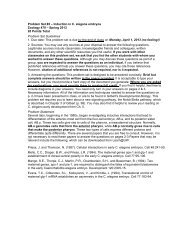
light microscopes have been made. Today, the instrument of
choice for light microscopy uses several lenses in combination
and is therefore called a compound microscope (Figure A-5).
Line of vision
Body tube
Objective
lenses
Specimen
Condenser
lenses
Illuminator
Base with
source of
illumination
Ocular lens
Path of light
(a) Principal parts and functions (b) The path of light (bottom to top)
Figure A-5 The Compound Light Microscope. (a) A compound light microscope. (b) The path
of light through the compound microscope.
Prism
The Light Microscope A-5

The optical path through a compound microscope, illustrated
in Figure A-5b, begins with a source of illumination, usually a
light source located in the base of the instrument. The light
rays from the source first pass through condenser lenses,
which direct the light toward a specimen mounted on a glass
slide and positioned on the stage of the microscope. The
objective lens, located immediately above the specimen, is
responsible for forming the primary image. Most compound
microscopes have several objective lenses of differing magnifications
mounted on a rotatable turret.
The primary image is further enlarged by the ocular
lens, or eyepiece. In some microscopes, an intermediate lens
is positioned between the objective and ocular lenses to
accomplish still further enlargement. You can calculate the
overall magnification of the image by multiplying the enlarging
powers of the objective lens, the ocular lens, and the
intermediate lens (if present). Thus, a microscope with a 10µ
objective lens, a 2.5µ intermediate lens, and a 10µ ocular lens
will magnify a specimen 250-fold.
The elements of the microscope described so far
create a basic form of light microscopy called brightfield
microscopy. Compared with other microscopes, the brightfield
microscope is inexpensive and simple to align and use.
However, the only specimens that can be seen directly by
brightfield microscopy are those that possess color or have
some other property that affects the amount of light that
passes through. Many biological specimens lack these characteristics
and must therefore be stained with dyes or examined
with specialized types of light microscopes. These special
microscopes have various advantages that make them especially
well suited for visualizing specific types of specimens.
These include phase-contrast microscopy, differential interference
contrast microscopy, fluorescence microscopy, and
confocal microscopy. We will look at these and several other
important techniques in the following sections.
PHASE-CONTRAST MICROSCOPY DETECTS
DIFFERENCES IN REFRACTIVE INDEX AND THICKNESS
As we will describe in more detail later, cells are often killed,
sliced into thin sections, and stained before being examined
by brightfield microscopy. While such procedures are useful
for visualizing the details of a cell’s internal architecture, little
can be learned about the dynamic aspects of cell behavior by
examining cells that have been killed, sliced, and stained.
Therefore, a variety of techniques have been developed for
using light microscopy to observe cells that are intact and, in
many cases, still living. One such technique, phase-contrast
microscopy, improves contrast without sectioning and staining
by exploiting differences in the thickness and refractive
index of various regions of the cells being examined. To
understand the basis of phase-contrast microscopy, we must
first recognize that a beam of light is made up of many individual
rays of light. As the rays pass from the light source
through the specimen, their velocity may be affected by the
physical properties of the specimen. Usually, the velocity of
the rays is slowed down to varying extents by different
regions of the specimen, resulting in a change in phase relative
to light waves that have not passed through the object.
A-6 Appendix Principles and Techniques of Microscopy
(Light waves are said to be traveling in phase when the crests
and troughs of the waves match each other.)
Although the human eye cannot detect such phase
changes directly, the phase-contrast microscope overcomes
this problem by converting phase differences into alterations
in brightness. This conversion is accomplished using a phase
plate (Figure A-6), which is an optical material inserted into
the light path above the objective lens to bring the direct or
undiffracted rays into phase with those that have been diffracted
by the specimen. The resulting pattern of wavelengths
intensifies the image, producing an image with highly contrasting
bright and dark areas against an evenly illuminated
background (Figure A-7). As a result, internal structures of
cells are often better visualized by phase-contrast microscopy
than with brightfield optics.
This approach to light microscopy is particularly useful
for examining living, unstained specimens because biological
materials almost inevitably diffract light. Phase-contrast
microscopy is widely used in microbiology and tissue culture
research to detect bacteria, cellular organelles, and other
small entities in living specimens.
Light source
Image plane
Phase
plate
Diffracted light
(phase altered
by specimen)
Objective lens
Direct light
(phase unaltered
by specimen)
Condenser lens
Annular
diaphragm
Figure A-6 Optics of the Phase-Contrast Microscope. The configuration
of the optical elements and the paths of light rays through
the phase-contrast microscope. Pink lines represent light diffracted
by the specimen, and black lines represent direct light.

50 m
Figure A-7 Phase-Contrast Microscopy. A phase-contrast micrograph
of epithelial cells. The cells were observed in an unprocessed
and unstained state, which is a major advantage of phase-contrast
microscopy.
DIFFERENTIAL INTERFERENCE CONTRAST (DIC)
MICROSCOPY UTILIZES A SPLIT LIGHT BEAM
TO DETECT PHASE DIFFERENCES
Differential interference contrast (DIC) microscopy resembles
phase-contrast microscopy in principle, but is more sensitive
because it employs a special prism to split the
illuminating light beam into two separate rays (Figure A-8).
When the two beams are recombined, any changes that
occurred in the phase of one beam as it passed through the
specimen cause it to interfere with the second beam. Because
the largest phase changes usually occur at cell edges (the
refractive index is more constant within the cell), the outline
of the cell typically gives a strong signal. The image appears
three-dimensional as a result of a shadow-casting illusion
that arises because differences in phase are positive on one
side of the cell but negative on the opposite side of the cell
(Figure A-9).
The optical components required for DIC microscopy
consist of a polarizer, an analyzer, and a pair of Wollaston
prisms (see Figure A-8). The polarizer and the first Wollaston
prism split a beam of light, creating two beams that are separated
by a small distance along one direction. After traveling
through the specimen, the beams are recombined by the second
Wollaston prism. If no specimen is present, the beams
recombine to form one beam that is identical to that which
initially entered the polarizer and first Wollaston prism. In
the presence of a specimen, the two beams do not recombine
in the same way (i.e., they interfere with each other), and the
resulting beam’s polarization becomes rotated slightly compared
with the original. The net effect is a remarkable
enhancement in resolution that makes this technique especially
useful for studying living, unstained specimens. As we
will see shortly, combining this technique with video
microscopy is an especially effective approach for studying
dynamic events within cells as they take place.
Other contrast enhancement methods are also used by
cell biologists. Hoffman modulation contrast, developed
Analyzer
(rotated 90° with respect to polarizer)
Wollaston prism
Specimen
Objective lens
Condenser lens
Wollaston prism
Polarizer
Light source
Image plane
Stage
2 beams of plane-polarized light,
separated by the prism below
Figure A-8 Optics of the Differential Interference Contrast (DIC)
Microscope. The configuration of the optical elements and the
paths of light rays through the DIC microscope.
10 m
Figure A-9 DIC Microscopy. A DIC micrograph of a cluster of rat
hippocampal neurons growing in culture. Notice the shadow-casting
illusion that makes these cells appear dark at the top and light
at the bottom.
The Light Microscope A-7

y Robert Hoffman, increases contrast by detecting optical
gradients across a transparent specimen using special filters
and a rotating polarizer. Hoffman modulation contrast
results in a shadow-casting effect similar to DIC microscopy.
FLUORESCENCE MICROSCOPY CAN DETECT
THE PRESENCE OF SPECIFIC MOLECULES
OR IONS WITHIN CELLS
Although the microscopic techniques described so far are
quite effective for visualizing cell structures, they provide relatively
little information concerning the location of specific
molecules. One way of obtaining such information is
through the use of fluorescence microscopy, which permits
fluorescent molecules to be located within cells. To understand
how fluorescence microscopy works, it is first necessary
to understand the phenomenon of fluorescence.
The Nature of Fluorescence. The term fluorescence refers to
a process that begins with the absorption of light by a molecule
and ends with its emission. This phenomenon is best
approached by considering the quantum behavior of light, as
opposed to its wavelike behavior. Figure A-10a is a diagram
of the various energy levels of a simple atom. When an atom
absorbs a photon (or quantum) of light of the proper energy,
one of its electrons jumps from its ground state to a higherenergy,
or excited, state. As the atom jiggles around, this electron
often loses some of its energy and drops back down to
the original ground state, emitting another photon as it does
so. The emitted photon is always of less energy (longer wavelength)
than the original photon that was absorbed. Thus, for
example, shining blue light on the atom may result in red
light being emitted. (The energy of a photon is inversely proportional
to its wavelength; therefore, red light, being longer
in wavelength than blue light, is lower in energy.)
Real fluorescent molecules have energy diagrams that
are more complicated than that depicted in Figure A-10a.
The number of possible energy levels in real molecules is
much greater, so the different energies that can be absorbed,
and emitted, are correspondingly greater. The absorption
and emission spectra of a typical fluorescent molecule are
shown in Figure A-10b. Every fluorescent molecule has its
own characteristic absorption and emission spectra.
The Fluorescence Microscope. Fluorescence microscopy is a
specialized type of light microscopy that employs light to excite
fluorescence in the specimen. A fluorescence microscope has an
exciter filter between the light source and the condenser lens
that transmits only light of a particular wavelength (Figure
A-11). The condenser lens focuses the light on the specimen,
causing fluorescent compounds in the specimen to emit light of
longer wavelength. Both the excitation light from the illuminator
and the emitted light generated by fluorescent compounds
in the specimen then pass through the objective lens. As the
light passes through the tube of the microscope above the
objective lens, it encounters a barrier filter that specifically
removes the excitation wavelengths. This leaves only the emission
wavelengths to form the final fluorescent image, which
therefore appears bright against a dark background.
A-8 Appendix Principles and Techniques of Microscopy
Energy of electron
Amount of light
Excited state
Photon
(a) Energy diagram
Ground state
Light absorbed Light emitted
400
500
600
Wavelength (nm)
(b) Absorption and emission spectra
Emitted photon
700
Figure A-10 Principles of Fluorescence. (a) An energy diagram of
fluorescence from a simple atom. Light of a certain energy is
absorbed (e.g., the blue light shown here). The electron jumps from
its ground state to an excited state. It returns to the ground state by
emitting a photon of lower energy and hence longer wavelength
(e.g., red light). (b) The absorption and emission spectra of a typical
fluorescent molecule. The blue curve represents the amount of
light absorbed as a function of wavelength, and the red curve shows
the amount of emitted light as a function of wavelength.
Fluorescent Antibodies. To use fluorescence microscopy for
locating specific molecules or ions within cells, researchers
must employ special indicator molecules called fluorescent
probes. A fluorescent probe is a molecule capable of emitting
fluorescent light that can be used to indicate the presence of a
specific molecule or ion.
One of the most common applications of fluorescent
probes is in immunostaining, a technique based on the ability
of antibodies to recognize and bind to specific molecules.
(The molecules to which antibodies bind are called antigens.)
Antibodies are proteins produced naturally by the immune
system in response to an invading microorganism, but they
can also be generated in the laboratory by injecting a foreign
protein or other macromolecule into an animal such as a
rabbit or mouse. In this way, it is possible to produce antibodies
that will bind selectively to virtually any protein that a
scientist wishes to study. Antibodies are not directly visible
using light microscopy, however, so they are linked to a fluorescent
dye such as fluorescein, which emits a green fluorescence,
or rhodamine, which emits a red fluorescence. More

Visible
light
Ultraviolet
light
Visible
light
Light source
Image plane
Specimen
Barrier filter
(blocks transmission of
all ultraviolet light, allowing
passage of only visible light)
Objective lens
Condenser lens
Exciter filter
(screens light and transmits
only ultraviolet rays)
Figure A-11 Optics of the Fluorescence Microscope.
The configuration of the optical elements and the paths of light
rays through the fluorescence microscope. Light from the source
passes through an exciter filter that transmits only excitation light
(solid black lines). Illumination of the specimen with this light
induces fluorescent molecules in the specimen to emit longerwavelength
light (blue lines). The barrier filter subsequently
removes the excitation light, while allowing passage of the emitted
light. The image is therefore formed exclusively by light emitted by
fluorescent molecules in the specimen.
recently, antibodies have been linked to “quantum dots,”
which are tiny light-emitting crystals that are chemically
more stable than traditional dyes. To identify the subcellular
location of a specific protein, cells are simply stained with a
fluorescent antibody directed against that protein and the
location of the fluorescence is then detected by viewing the
cells with light of the appropriate wavelength.
Immunofluorescence microscopy can be performed using
antibodies that are directly labeled with a fluorescent dye
(Figure A-12a). However, immunofluorescence microscopy is
more commonly performed using indirect immunofluorescence
(Figure A-12b). In indirect immunofluorescence, a
tissue or cell is treated with an antibody that is not labeled with
dye. This antibody, called the primary antibody, attaches to
specific antigenic sites within the tissue or cell. A second type
of antibody, called the secondary antibody, is then added. The
secondary antibody is labeled with a fluorescent dye, and it
attaches to the primary antibody. Because more than one primary
antibody molecule can attach to an antigen, and more
Specific antibodies
against antigen
(a) Immunofluorescence
Specific antibodies
against antigen
(primary antibody)
Antibodies labeled
with fluorescent dye
(b) Indirect immunofluorescence
Allow antibodies
to bind to antigen
Allow antibodies
to bind to antigen
Add labeled antibodies
that bind to primary
antibodies ("secondary
antibody")
Figure A-12 Immunostaining Using Fluorescent Antibodies.
Immunofluorescence microscopy relies on the use of fluorescently
labeled antibodies to detect specific molecular components (antigens)
within a tissue sample. (a) In direct immunofluorescence, an
antibody that binds to a molecular component in a tissue sample is
labeled with a fluorescent dye. The labeled antibody is then added
to the tissue sample, and it binds to the tissue in specific locations.
The pattern of fluorescence that results is visualized using fluorescence
or confocal microscopy. (b) In indirect immunofluorescence,
a primary antibody is added to the tissue. Then a secondary antibody
that carries a fluorescent label is added. The secondary antibody
binds to the primary antibody. Because more than one
fluorescent secondary antibody can bind to each primary molecule,
indirect immunofluorescence effectively amplifies the fluorescent
signal, making it more sensitive than direct immunofluorescence.
than one secondary antibody molecule can attach to each primary
antibody, more fluorescent molecules are concentrated
near each molecule that we seek to detect. As a result, indirect
immunofluorescence results in signal amplification, and it is
much more sensitive than the use of a primary antibody alone.
The method is “indirect” because it does not examine where
antibodies are bound to antigens; technically, the fluorescence
reflects where the secondary antibody is located. This, of
course, provides an indirect measure of where the original
molecule of interest is located.
Other Fluorescent Probes. Naturally occurring proteins that
selectively bind to specific cell components are also used in
fluorescence microscopy. For example, Figure A-13 shows the
The Light Microscope A-9

10 m
Figure A-13 Fluorescence Microscopy. Cultured dog kidney
epithelial cells stained with the fluorescent stain phalloidin, which
binds to actin microfilaments.
fluorescence image of epithelial cells stained with a fluorescein-tagged
mushroom toxin, phalloidin, which binds specifically
to actin microfilaments. Another powerful fluorescence
technique utilizes the Green Fluorescent Protein (GFP), a naturally
fluorescent protein made by the jellyfish Aequoria victoria.
Using recombinant DNA techniques, scientists can fuse
DNA encoding GFP to a gene coding for a particular cellular
protein. The resulting recombinant DNA can then be introduced
into cells, where it is expressed to produce a fluorescent
version of the normal cellular protein. In many cases, the
fusion of GFP to the end of a protein does not interfere with its
function, allowing the use of fluorescence microscopy to view
the GFP-fusion protein as it functions in a living cell (Figure
A-14). Molecular biologists have produced mutated forms of
(a) 00:00 (b) 03:40 (c) 05:08
Figure A-14 Using Green Fluorescent Protein to Visualize Proteins. An image series of
a living, one-cell nematode worm embryo undergoing mitosis. The embryo is expressing
b-tubulin
that is tagged with the green fluorescent protein (GFP). Elapsed time
from the first frame is shown in minutes:seconds.
A-10 Appendix Principles and Techniques of Microscopy
GFP that absorb and emit light at a variety of wavelengths. In
addition, other naturally fluorescent proteins have been identified,
such as a red fluorescent protein from coral. These tools
have expanded the repertoire of fluorescent molecules at the
disposal of cell biologists.
In addition to detecting macromolecules such as proteins,
fluorescence microscopy can also be used to monitor
the subcellular distribution of various ions. To accomplish
this task, chemists have synthesized molecules whose fluorescent
properties are sensitive to the concentrations of ions
such as and Mg as well as to the electri-
2; Ca ,
2; , H ; , Na ; , Zn2; ,
cal potential across the plasma membrane. When these fluorescent
probes are injected into cells in a form that becomes
trapped in the cytosol or in a specific intracellular component,
they provide important information about the ionic
conditions inside the cell. For example, a fluorescent probe
called fura-2 is commonly used to track the Ca concentration
inside living cells, because fura-2 emits a yellow fluores-
2;
cence in the presence of low concentrations of and a
Ca 2;
green and then blue fluorescence in the presence of progressively
higher concentrations of this ion. Therefore, monitoring
the color of the fluorescence in living cells stained with
this probe allows scientists to observe changes in the intracellular
Ca concentration as they occur.
2;
CONFOCAL MICROSCOPY MINIMIZES BLURRING BY
EXCLUDING OUT-OF-FOCUS LIGHT FROM AN IMAGE
When intact cells are viewed, the resolution of fluorescence
microscopy is limited by the fact that although fluorescence
is emitted throughout the entire depth of the specimen, the
viewer can focus the objective lens on only a single plane at
any given time. As a result, light emitted from regions of the
specimen above and below the focal plane cause a blurring of
the image (Figure A-15a). To overcome this problem, cell
biologists often turn to the confocal microscope—a specialized
type of light microscope that employs a laser beam to
produce an image of a single plane of the specimen at a time
(Figure A-15b). This approach improves the resolution along
the optical axis of the microscope—that is, structures in the
10 m

(a) Traditional fluorescence microscopy (b) Confocal fluorescence microscopy 25 m
Figure A-15 Comparison of Confocal Fluorescence Microscopy with Traditional Fluorescence
Microscopy. These fluorescence micrographs show fluorescently labeled glial cells (red) and
nerve cells (green) stained with two different fluorescent markers. (a) In traditional
fluorescence microscopy, the entire specimen is illuminated, so fluorescent material above
and below the plane of focus tends to blur the image. (b) In confocal fluorescence
microscopy, incoming light is focused on a single plane, and out of focus fluorescence from
the specimen is excluded. The resulting image is therefore much sharper. (Image Courtesy:
Karl Garsha, Digital Light Microscopy Specialist, Imaging Technology Group, Beckman
Institute for Advanced Science and Technology, University of Illinois at Urbana-Champaign,
Urbana, IL www.tig.uiux.edu.)
middle of a cell may be distinguished from those on the top
or bottom. Likewise, a cell in the middle of a piece of tissue
can be distinguished from cells above or below it.
To understand this type of microscopy, it is first necessary
to consider the paths of light taken through a simple
lens. Figure A-16 illustrates how a simple lens forms an image
of a point source of light. To understand what your eye
would see, imagine placing a piece of photographic film in
the plane of focus (image plane). Now ask how the images of
other points of light placed further away or closer to the lens
contribute to the original image (Figure A-16b). As you
might guess, there is a precise relationship between the distance
of the object from the lens (o), the distance from the
lens to the image of that object brought into focus (i), and
the focal length of the lens ( f ). This relationship is given by
the equation
1
f = 1 1
o +
i .
(A-5)
As Figure A-16b shows, light arising from the points that are
not in focus covers a greater surface area on the film because
the rays are still either converging or diverging. Thus, the
image on the film now has the original point source that is in
focus, with a superimposed halo of light from the out-offocus
objects.
If we were only interested in seeing the original point
source, we could mask out the extraneous light by placing
an aperture, or pinhole, in the same plane as the film. This
principle is used in a confocal microscope to discriminate
against out-of-focus rays. In a real specimen, of course, we do
not have just a single extraneous source of light on each side
of the object we wish to see, but a continuum of points. To
understand how this affects our image, imagine that instead
of three points of light, our specimen consists of a long thin
tube of light, as in Figure A-16c. Now consider obtaining an
image of some arbitrary small section, dx. If the tube sends
out the same amount of light per unit length, then even with
a pinhole, the image of interest will be obscured by the halos
arising from other parts of the tube. This occurs because
there is a small contribution from each out-of-focus section,
and the sheer number of small sections will create a large
background over the section of interest.
This situation is very close to that which we face when
dealing with real biological samples that have been stained
with a fluorescent probe. In general, the distribution of the
probe is three-dimensional, and when we wish to look at the
detail of a single object (such as a microtubule) using conventional
fluorescence microscopy, the image is often marred
by the halo of background light that arises mostly from
microtubules above and below the plane of interest. To circumvent
this, we can preferentially illuminate the plane of
interest, thereby biasing the contributions in the image plane
so that they arise mostly from a single plane (Figure A-16d).
Thus, the essence of confocal microscopy is to bring the illumination
beam that excites the fluorescence into focus in a
single plane, and to use a pinhole to ensure that the light we
The Light Microscope A-11

Point
of light
Lens
Image plane
View of
image plane
(a) Formation of an image of a single point of light by a lens
3 points
of light
Lens
Image plane
View of
image plane
(b) Formation of an image of a point of light in the presence
of two other points
dx
Tube
of light
Lens Image plane
(c) Formation of an image of a section of an equally bright
tube of light
dx
Lens Image plane
(d) Formation of an image of a brightened section of a
tube of light
View of
image plane
View of
image plane
collect in the image plane arises mainly from that plane of
focus.
Figure A-17 illustrates how these principles are put to
work in a laser scanning confocal microscope, which illuminates
specimens using a laser beam focused by an objective
lens down to a diffraction-limited spot. The position of the
A-12 Appendix Principles and Techniques of Microscopy
Figure A-16 Paths of Light Through a Single Lens. (a) The image of
a single point of light formed by a lens. (b) The paths of light from
three points of light at different distances from the lens. In the
image plane, the in-focus image of the central point is superimposed
with the out-of-focus rays of the other points. A pinhole
or aperture around the central point can be used to discriminate
against out-of-focus rays and maximize the contributions from the
central point. (c) The paths of light originating from a continuum
of points, represented as a tube of light. This is similar to a uniformly
illuminated sample. In the image plane, the contributions
from an arbitrarily small in-focus section, dx, are completely
obscured by the other out-of-focus rays; here a pinhole does not
help. (d) By illuminating only a single section of the tube strongly
and the rest weakly, we can recover information in the image plane
about the section dx. Now a pinhole placed around the spot will
reject out-of-focus rays. Because the rays in the middle are almost
all from dx, we have a means of discriminating against the dimmer,
out-of-focus points.
spot is controlled by scanning mirrors, which allow the beam
to be swept over the specimen in a precise pattern. As the
beam is scanned over the specimen, an image of the specimen
is formed in the following way. First, the fluorescent
light emitted by the specimen is collected by the objective
lens and returned along the same path as the original incoming
light. The path of the fluorescent light is then separated
from the laser light using a dichroic mirror, which reflects one
color but transmits another. Because the fluorescent light has
a longer wavelength than the excitation beam, the fluorescence
color is shifted toward the red. The fluorescent light
passes through a pinhole placed at an image plane in front of
a photomultiplier tube, which acts as a detector. The signal
from the photomultiplier tube is then digitized and displayed
by a computer. To see the enhanced resolution that results
from confocal microscopy, look back to Figure A-15, which
shows images of the same cell visualized by conventional
fluorescence microscopy and by laser scanning confocal
microscopy.
As an alternative to laser scanning confocal microscopy,
a spinning disc confocal microscope uses rapidly spinning discs
containing a series of small lenses and a corresponding series
of pinholes. Although it cannot produce optical sections
as thin as laser scanning microscopes can produce, it can
generate confocal images that can be acquired rapidly using
sensitive digital cameras. Such speed is useful for visualizing
very rapid events within cells.
In confocal microscopy, a pinhole is used to exclude outof-focus
light. The result is a sharp image, but molecules
above and below the focal plane of the objective lens are still
being excited by the incoming light. This can result in rapid
bleaching of the fluorescent molecules; in some cases, especially
when viewing living cells that contain fluorescent molecules,
such bleaching releases toxic radicals that can cause
the cells to die. To reduce such “photodamage,” it would
be desirable if only the fluorescent molecules very close to
the focal plane being examined were excited. This is possible
using multiphoton excitation microscopy. In multiphoton
excitation microscopy, a laser that emits pulses of light very
rapidly and with very high energy is used to irradiate the

(a)
To
computer
Image plane
Detector
(photomultiplier tube)
(b)
Pinhole
Laser
Dichroic mirror
Objective lens
Specimen
Scanning
mirrors
Figure A-17 A Laser Scanning Confocal Microscope. (a) A
photograph and (b) a schematic of a laser scanning confocal
microscope. A laser is used to illuminate one spot at a time in the
specimen (blue lines). The scanning mirrors move the spot in a
given plane of focus through a precise pattern. The fluorescent light
that is emitted from the specimen (red lines) bounces off the same
scanning mirrors and returns along the original path of the illumination
beam. The emitted light does not return to the laser, but
instead is transmitted through the dichroic mirror (which in this
example reflects blue light but transmits red light). A pinhole in the
image plane blocks the extraneous rays that are out of focus. The
light is detected by a photomultiplier tube, the signal from which is
digitized and stored by a computer.
specimen. Two (or in some cases, three or more) photons
must be absorbed by a fluorescent molecule in quick succession
in order for it to fluoresce (Figure A-18). The likelihood
of this happening is very low, except near the focal plane of
the objective lens. As a result, only the fluorescent molecules
that are in focus fluoresce. The result is very similar in sharpness
to confocal microscopy, but no pinhole is needed,
as there is no out-of-focus light that needs to be excluded.
Photodamage is also dramatically reduced. As an example,
multiphoton excitation microscopy was used to image the
living embryo shown in Figure A-14.
A third technique, digital deconvolution microscopy,
can be used to provide very sharp images. Digital deconvolution
relies on a completely different principle. In this case,
normal fluorescence microscopy is used to acquire a series of
images throughout the thickness of a specimen. Then a computer
is used to digitally process, or deconvolve, each focal
plane to mathematically remove the contribution due to the
out-of-focus light. In many cases, digital deconvolution can
produce images that are comparable to those obtained by
confocal microscopy (Figure A-19). One advantage of deconvolution
is that the microscope is not restricted to the specific
wavelengths of light used in the lasers commonly found
in confocal microscopes.
DIGITAL VIDEO MICROSCOPY CAN RECORD
ENHANCED TIME-LAPSE IMAGES
The advent of solid-state light detectors has, in many circumstances,
made it possible to replace photographic film with
an electronic equivalent—that is, with a video camera or digital
imaging camera. These developments have given rise to
the technique of digital video microscopy, in which microscopic
images are recorded and stored electronically by placing
a video camera in the image plane produced by the
ocular lens. This approach takes advantage of the fact that
video cameras can detect subtle differences in contrast better
than the human eye. In addition, video cameras generate
images in a digital form that can be enhanced by computer
processing. In the enhancing process, the signal from the
camera is first stored as a two-dimensional array of numbers
whose values correspond to the lightness or darkness at particular
locations in the image. The data are then processed by
computer to increase contrast and remove background features
that obscure the image of interest (Figure A-20).
The resulting enhancement allows the visualization of
structures that are an order of magnitude smaller than can
be seen with a conventional light microscope. As we have
seen, conventional light microscopy is generally incapable of
resolving objects smaller than 200 nm in diameter. Computerenhanced
video microscopy, by contrast, permits the visualization
of individual microtubules, which measure only 25 nm in
diameter. Digital video techniques can be applied to conventional
brightfield light microscopy, as well as to DIC and fluorescence
microscopy, thereby creating a powerful set of
approaches for improving the effectiveness of light microscopy.
An additional advantage of digital video microscopy is
that the specimen does not need to be killed by fixation, as is
required with electron microscopy, so dynamic events can be
monitored as they take place. Moreover, special intensified
video cameras have been developed that can detect extremely
dim images, thereby facilitating the ability to record a rapid
series of time-lapse pictures of cellular events as they proceed.
For example, with conventional photographic film, it
may take a minute or more to record the image of a fluorescently
labeled cell, which means that a time-lapse series of
photographs can only show one picture of the cell per
minute. But an intensified video camera can record an image
The Light Microscope A-13

(a) Confocal microscropy (a) Multiphoton microscopy
(a) (b)
Figure A-19 Digital Deconvolution Microscopy. A fission yeast cell stained with a dye
specific for DNA (red) and a membrane-specific dye (green). The image on the left is
an unprocessed optical section through the center of the cell. The image on the right is
a projection of all the sections following three-dimensional image processing. The ring
of the developing medial septum (red) is forming between the two nuclei (red) that
arose by nuclear division during the previous mitosis.
of the same cell 30 times per second, making it possible to
monitor rapid changes in the appearance and behavior of
subcellular components. This has allowed scientists to obtain
information on the changes in concentration and subcellular
distribution of such cytosolic components as second messengers
during cellular signaling, and to study the role of
cytoskeletal structures in intracellular movements. Thus,
digital video microscopy has greatly expanded our ability to
monitor events as they occur within living cells.
A-14 Appendix Principles and Techniques of Microscopy
Figure A-18 Multiphoton Excitation
Microscopy. (a) In a standard laser
scanning confocal microscope, the
laser results in fluorescence in an
hourglass-shaped path throughout
the specimen. Because a large area
fluoresces, photodamage is much
more likely to occur than in
multiphoton excitation microscopy.
(b) In a multiphoton excitation
microscope, fluorescence is limited
to a spot at the focus of the pulsed
infrared laser beam, resulting in
much less damage. The infrared
illumination also penetrates more
deeply into the specimen than
visible light.
4 m
Digital microscopy is not only useful for examining events
in one focal plane. In a variation of this technique, a computer
is used to control a focus motor attached to a microscope.
Images are then collected throughout the thickness of a
specimen. When such a series of images is collected at specific
time intervals, such microscopy is called four-dimensional
microscopy (this phrase is borrowed from physics; the four
dimensions are the three dimensions of space plus the additional
dimension of time). Analyzing four-dimensional data

(a) (b) (c) (d)
Figure A-20 Computer-Enhanced Digital
Video Microscopy. This series of micrographs
shows how computers can be used
to enhance images obtained with light
microscopy. In this example, an image of
several microtubules, which are too small to
requires special computer software that can navigate between
focal planes over time to display specific images.
OPTICAL METHODS CAN BE USED TO MEASURE
THE MOVEMENTS AND PROPERTIES OF PROTEINS
AND OTHER MACROMOLECULES
Optical microscopy can be used to help us visualize where molecules
reside within cells and to study the dynamic movements
and properties of biological molecules. We briefly consider
these modern techniques in this section.
Photobleaching and photoactivation. When fluorescent
molecules are irradiated with light at the appropriate excitation
wavelength for long periods of time, they undergo
photobleaching (i.e., the irradiation induces the molecules
to cease fluorescing). If a cell is only exposed to intense light
in a small region, such bleaching results in a characteristic
decrease in fluorescence (Figure A-21a). As unbleached
molecules move into the bleach zone, the fluorescence gradually
returns to normal levels. Such fluorescence recovery after
photobleaching (FRAP) is therefore one useful measure of
how fast molecules diffuse or undergo directed transport
(see Figure 7-11 on p. 167 for a classic example of the use of
FRAP).
In other cases, fluorescent molecules are chemically
modified so that they do not fluoresce until they are irradiated
with a specific wavelength of light, usually ultraviolet
light. The UV light induces the release of the chemical modifier,
allowing the molecule of interest to fluoresce. Both
chemically modified dyes and forms of GFP have been produced
that behave in this way. Such compounds are often
called caged compounds, because they are only “freed” by this
light-induced cleavage. Uncaging, or photoactivation, produces
the converse situation to photobleaching: local
uncaging of a fluorescent molecule produces a bright spot of
fluorescence that can be followed as the molecules make their
way throughout the cell (Figure A-21b). Uncaging via
be seen with unenhanced light microscopy,
are processed to make them visible in detail.
(a) The image resulting from electronic
contrast enhancement of the original image
(which appeared to be empty). (b) The
background of the enhanced image in (a),
2.5 m
which is then (c) subtracted from image (a),
leaving only the microtubules. (d) The final,
detailed image resulting from electronic
averaging of the separate images processed
as shown in a–c.
photoactivation can also be used to convert other kinds of
inert molecules to their active state. For example, “caged calcium”
is actually a calcium chelator that is bound to calcium
ions. When the caged compound is irradiated, it gives up its
calcium, causing a local elevation of calcium within the cell.
Total internal reflection fluorescence microscopy. An even
more spatially precise method for observing fluorescent molecules
involves total internal reflection fluorescence (TIRF)
microscopy. TIRF relies on a useful property of light: when
light moves from a medium with a high refractive index (such
as glass) to a medium with a lower refractive index (such as
water or a cell), if the angle of incidence of the light exceeds a
certain angle (called the critical angle), the light is reflected.
You may be familiar with fiber-optic cables, which rely on the
very same physical principle. The curvature of the fiber causes
almost all of the light that passes into the cable to be internally
reflected, allowing such fibers to serve as “light pipes.” Microscopists
can use special lenses to exploit total internal reflection
as well. When fluorescent light shines on a cell such that
all of the light exceeds the critical angle, it will undergo total
internal reflection. If all of the light is reflected, why is TIRF
useful? It turns out that a very small layer of light, called the
“evanescent field,” extends into the water or cell (Figure
A-21c). This layer is very thin, about 100 nm, making TIRF up
to ten times better than a confocal microscope for resolving
small objects very close to the surface of a coverslip. This
makes TIRF extremely useful for studying the release of secretory
vesicles, or for observing the polymerization of actin.
Fluorescence resonance energy transfer. Fluorescence microscopy
is useful not only for observing the movements of
proteins, but also for measuring their physical interactions
with one another. When two fluorescent molecules whose fluorescence
properties are matched are brought very close to one
another, it is possible for them to experience fluorescence
resonance energy transfer (FRET). In FRET, illuminating a
The Light Microscope A-15

(a) Photobleaching
(b) Photoactivation
Water
(low index
of refraction)
(c)
Immersion
oil
100 nm
“Evanescent
field”
Gactin
monomer
Objective
lens
Glass
(high index
of refraction)
Figure A-21 Techniques for studying dynamic movements of molecules
within cells. (a) Photobleaching of fluorescent molecules. A
well-defined area of a cell is irradiated, causing bleaching of fluorescent
molecules. Gradually, new, unbleached molecules invade the
bleached zone. (b) Photoactivation of fluorescent proteins. Photoactivation
of a selected region, such as the nucleus (indicated in red),
results in an increase in fluorescence. The subsequent movements of
the fluorescent molecules can then be monitored. (c) Total internal
reflection fluorescence (TIRF) microscopy. The example shown here
involves fluorescent G actin monomers. (see Chapter 15). When a
beam of light in a medium of high refractive index (such as glass)
strikes an interface with a medium of lower refractive index (such as
a cell or water) at an angle that exceeds the critical angle (a), it
undergoes total internal reflection. Total internal reflection results in
an “evanescent field” in the medium of lower refractive index, which
falls off quickly with distance. This allows only a very small number
of fluorescent molecules to be seen.
cell at the excitation wavelength of the first, or donor, fluorophore
results in energy transfer to the second, or acceptor,
fluorophore. This energy transfer does not itself involve a photon
of light, but once it occurs, it causes the acceptor to emit
light at its characteristic wavelength. A commonly used pair of
fluorescent molecules used in FRET is derived from GFP: one
glows with bluish (cyan) fluorescence (it is often called cyan
fluorescent protein, or CFP); the other is excited by bluish light
and glows with a yellowish color (so it is called yellow
fluorescent protein, or YFP). FRET can be measured between
two separate proteins (intermolecular FRET; Figure A-22a), or
between fluorescent side chains on the same protein
(intramolecular FRET; Figure A-22b). FRET only acts at a very
short range; as a result, intermolecular FRET provides a
A-16 Appendix Principles and Techniques of Microscopy
(a)
(b)
(c)
CFP
Proteins interact
YFP
Cell-signaling
event
0 min 5 min 30 min
FRET occurs:
incoming light
is absorbed by
CFP; YFP emits
yellow light
FRET
occurs
Ras
activity:
high
Figure A-22 Fluorescence resonance energy transfer (FRET). (a)
Intermolecular FRET. When two proteins attached to two different
fluorescent side chains (such as cyan fluorescent protein, or CFP,
and yellow fluorescent protein, or YFP) are in close proximity, the
CFP can transfer energy directly to the YFP when the CFP is
excited. The YFP then fluoresces, and this fluorescence can be
measured. (b) Intramolecular FRET. In this case, CFP and YFP are
attached to the same molecule, but they can only interact when the
protein undergoes a conformational change. Such engineered
proteins can be used as cellular “biosensors.” (c) Detecting Ras
activation in a living cell. A COS-1 cell expressing a protein that
undergoes intramolecular FRET in regions where Ras is active
shows an increase in FRET after the cell is exposed to epidermal
growth factor (EGF), which activates Ras.
readout regarding where within a cell two fluorescent proteins
are essentially touching one another.
Intramolecular FRET is used in several kinds of “molecular
biosensors.” We saw one example of such a biosensor in
Chapter 14, when we considered “cameleons.” These engineered
proteins change shape to bring blue and yellow fluorescent protein
subunits into contact only when calcium levels rise. The
resulting FRET can be used to measure local calcium levels.
Similar biosensors are being used to measure the local activation
of small G proteins, such as Ras, a key regulator of receptor
tyrosine kinase signaling (see Chapter 14). These sensors
undergo a change in shape that allows FRET only in regions of
the cell in which the normal Ras is activated (Figure A-22c).
low

Figure A-23 “Optical tweezers.” A small plastic bead can be held
in place by a laser beam focused through the objective lens of a
microscope. When the bead is attached to a molecule such as
myosin, the force produced by the myosin as it pulls on an actin
filament attached to a microscope slide can be precisely measured.
“Optical tweezers.” The final application of light microscopy
we will discuss may seem a bit like science fiction, but it actually
relies on well-established ways in which light interacts with
small objects. When photons strike small objects, they exert
“light pressure” on them. When a small object is highly curved,
such as a small plastic bead, the differential forces exerted by
a tightly focused laser beam channeled through a microscope
tend to cause the bead to remain in the center of the beam,
trapping it via light pressure. Such “optical tweezers” can be
used to move objects, or they can be used to exert exceedingly
small forces on beads that are attached to proteins or other
molecules. By measuring the forces exerted on beads coupled
to myosin, for example, scientists have been able to measure
the forces produced by the power stroke of a single myosin
protein (Figure A-23).
Sample Preparation Techniques
for Light Microscopy
One of the attractive features of light microscopy is the ease
with which most specimens can be prepared for examination.
In some cases, sample preparation involves nothing
more than mounting a small piece of the specimen in a suitable
liquid on a glass slide and covering it with a glass coverslip.
The slide is then positioned on the specimen stage of the
microscope and examined through the ocular lens, or with a
camera.
However, to take maximum advantage of the resolving
power of the light microscope, samples are usually prepared
in a way designed to enhance contrast—that is, differences
in the darkness or color of the structures being
examined. A common means for enhancing contrast is to
apply specific dyes that color or otherwise alter the lighttransmitting
properties of cell constituents. Preparing cells
for staining typically involves special procedures, as we
now describe.
SPECIMEN PREPARATION OFTEN INVOLVES
FIXATION, SECTIONING, AND STAINING
To prepare cells for staining, tissues are first treated with
fixatives that kill the cells while preserving their structural
appearance. The most widely employed fixatives are acids and
aldehydes such as acetic acid, picric acid, formaldehyde, and
glutaraldehyde. One way of fixing tissues is simply to immerse
them in the fixative solution. An alternative approach for animal
tissues is to inject the fixative into the bloodstream of the
animal before removing the organs. This technique, called
perfusion, may help reduce artifacts, which are false or inaccurate
representations of the specimen that result from chemical
treatment or handling of the cells or tissues.
In most cases, the next step is to slice the specimen into
sections that are thin enough to transmit light. Otherwise, the
specimen will appear opaque under the microscope and little
discernible structure will be visible. To prepare such thin sections,
the specimen is embedded in a medium (such as plastic
or paraffin wax) that can hold it rigidly in position while sections
are cut. Since paraffin is insoluble in water, any water in
the specimen must first be removed (by dehydration in alcohol,
usually) and replaced by an organic solvent, such as
xylene, in which paraffin is soluble. The processed tissue is
then placed in warm, liquefied paraffin and allowed to harden.
Dehydration is less critical if the specimen is embedded in a
water-soluble medium instead of paraffin. Specimens may also
be embedded in epoxy plastic resin, or as an alternative way of
providing support, the tissue can simply be quick-frozen.
After embedding or quick-freezing, the specimen is
sliced into thin sections a few micrometers thick by using a
microtome, an instrument that operates somewhat like a
meat slicer (Figure A-24). The specimen is simply mounted
Microtome
arm
Specimen embedded
in paraffin wax or
plastic resin
Metal or glass blade
Ribbon of
thin sections
Ribbons of sections on
glass slide, stained
and mounted under
a coverslip.
Figure A-24 Sectioning with a Microtome. The fixed specimen is
embedded in paraffin wax or plastic resin and mounted on the arm
of the microtome. As the arm moves up and down through a circular
arc, the blade cuts successive sections. The sections adhere to
each other, forming a ribbon of thin sections that can be mounted
on a glass slide, stained, and protected with a coverslip.
Sample Preparation Techniques for Light Microscopy A-17

on the arm of the microtome, which advances the specimen
by small increments toward a metal or glass blade that slices
the tissue into thin sections. As successive sections are cut,
they usually adhere to one another, forming a ribbon of thin
sections. These sections are then mounted on a glass slide
and subjected to staining with any of a variety of dyes that
have been adapted for this purpose. Sometimes the tissue is
treated with a single stain, but more often a series of stains is
used, each with an affinity for a different kind of cellular
component. Once stained, the specimen is covered with a
glass coverslip for protection.
A historically important approach for localizing specific
components within cells is microscopic autoradiography, a
technique that uses photographic emulsion to determine
where a specific radioactive compound is located within a cell
at the time the cell is fixed and sectioned for microscopy. In
this procedure, radioactive compounds are incubated with
tissue sections or administered to intact cells or organisms.
After sufficient time has elapsed for the radioactive compound
to become incorporated into newly forming intracellular
molecules and structures, the remaining unincorporated
radioactivity is washed away and the specimen is sectioned in
the conventional way and mounted on a microscope slide.
The slide is then covered with a thin layer of photographic
emulsion and placed in a sealed box for the desired
length of time, often for several days or even weeks. When the
emulsion is later developed and the specimen is examined
under the microscope, silver grains appear directly above the
specimen wherever radiation had bombarded the emulsion.
The location of these silver grains, which are readily visible
(a)
Figure A-25 A Transmission Electron Microscope. (a) A photograph
and (b) a schematic diagram of a TEM.
A-18 Appendix Principles and Techniques of Microscopy
with both the light and electron microscope, can be used to
pinpoint the region of the cell containing the radioactivity.
The Electron Microscope
The impact of electron microscopy on our understanding of
cells can only be described as revolutionary. Yet, like light
microscopy, electron microscopy has both strengths and
weaknesses. In electron microscopy, resolution is much better,
but specimen preparation and instrument operation are often
more difficult. Electron microscopes are of two basic designs:
the transmission electron microscope and the scanning electron
microscope. Scanning and transmission electron microscopes
are similar in that each employs a beam of electrons to produce
an image. However, the instruments use quite different
mechanisms to form the final image, as we see next.
TRANSMISSION ELECTRON MICROSCOPY
FORMS AN IMAGE FROM ELECTRONS THAT
PASS THROUGH THE SPECIMEN
The most commonly used type of electron microscope is
called the transmission electron microscope (TEM) because
it forms an image from electrons that are transmitted
through the specimen being examined. As shown in Figure
A-25, most of the parts of the TEM are similar in name and
function to their counterparts in the light microscope,
although their physical orientation is reversed. We will look
briefly at each of the major features.
Specimen
Specimen
stage
Detector
(b)
Cathode (tungsten
filament)
Anode
First
condenser
lens
Second
condenser
lens
Objective lens
Intermediate lens
Projector lens
Electron gun
(inside cylinder,
not shown)
Condenser
lens system

The Vacuum System and Electron Gun. Because electrons
cannot travel very far in air, a strong vacuum must be maintained
along the entire path of the electron beam. Two types
of vacuum pumps work together to create this vacuum. On
some TEMs, a device called a cold trap is incorporated into
the vacuum system to help establish a high vacuum. The cold
trap is a metal insert in the column of the microscope that is
cooled by liquid nitrogen. The cold trap attracts gases and
random contaminating molecules, which then solidify on the
cold metal surface.
The electron beam in a TEM is generated by an electron
gun, an assembly of several components. The cathode, a
tungsten filament similar to a light bulb filament, emits electrons
from its surface when it is heated. The cathode tip is
near a circular opening in a metal cylinder. A negative voltage
on the cylinder helps control electron emission and shape the
beam. At the other end of the cylinder is the anode. The
anode is kept at 0 V, while the cathode is maintained at
50–100 kV. This difference in voltage causes the electrons to
accelerate as they pass through the cylinder and hence is
called the accelerating voltage.
Electromagnetic Lenses and Image Formation. The formation
of an image using electron microscopy depends on both
the wavelike and the particle-like properties of electrons.
Because electrons are negatively charged particles, their
movement can be altered by magnetic forces. This means
that the trajectory of an electron beam can be controlled
using electromagnets, just as a glass lens can bend rays of
light that pass through it.
As the electron beam leaves the electron gun, it enters a
series of electromagnetic lenses (Figure A-25b). Each lens is
simply a space influenced by an electromagnetic field. The
focal length of each lens can be increased or decreased by
varying the amount of electric current applied to its
energizing coils. Thus, when several lenses are arranged
together, they can control illumination, focus, and
magnification.
The condenser lens is the first lens to affect the electron
beam. It functions in the same fashion as its counterpart
in the light microscope to focus the beam on the
specimen. Most electron microscopes actually use a condenser
lens system with two lenses to achieve better focus of
the electron beam. The next component, the objective lens,
is the most important part of the electron microscope’s
sophisticated lens system. The specimen is positioned
on the specimen stage within the objective lens. The objective
lens, in concert with the intermediate lens and the
projector lens, produces a final image on a viewing screen
that fluoresces when struck by electrons or that is produced
directly by a detector.
How is an image formed from the action of these electromagnetic
lenses on an electron beam? Recall that the electron
beam generated by the cathode passes through the
condenser lens system and impinges on the specimen. When
the beam strikes the specimen, some electrons are scattered
by the sample, whereas others continue in their paths
relatively unimpeded. This scattering of electrons is the result
of properties created in the specimen by preparation
procedures we will describe shortly. Specimen preparation, in
other words, imparts selective electron density to the specimen;
that is, some areas become more opaque to electrons
than others. Electron-dense areas of the specimen will appear
dark because few electrons pass through, whereas other areas
will appear lighter because they permit the passage of more
electrons.
The contrasting light, dark, and intermediate areas of
the specimen create the final image. The fact that the image is
formed by differing extents of electron transmission through
the specimen is reflected in the name transmission electron
microscope.
The Image Capture System. Since electrons are not visible
to the human eye, the final image is detected in the transmission
electron microscope by allowing the transmitted
electrons to strike a fluorescent screen or photographic
film. The use of film allows one to create a photographic
print called an electron micrograph, which then becomes a
permanent photographic record of the specimen (Figure
A-26a). In many modern microscopes, a digital camera
records the screen or a digital detector directly detects
incoming electrons.
Voltage. An electron beam is too weak to penetrate very
far into biological samples, so specimens examined by conventional
transmission electron microscopy must be
extremely thin (usually no more than 100 nm in thickness).
Otherwise, the electrons will not be able to pass through the
specimen and the image will be entirely opaque. The examination
of thicker sections requires a special high-voltage
electron microscope (HVEM), which is similar to a transmission
electron microscope but utilizes an accelerating
voltage that is much higher—about 200–1000 kV compared
with the 50–100 kV of a TEM. Because the penetrating
power of the resulting electron beam is roughly ten times as
great as that of conventional electron microscopes, relatively
thick specimens can be examined with good resolution.
As a result, cellular structure can be studied in sections
as thick as 1 mm,
about ten times the thickness possible with
an ordinary TEM.
SCANNING ELECTRON MICROSCOPY
REVEALS THE SURFACE ARCHITECTURE
OF CELLS AND ORGANELLES
Scanning electron microscopy is a fundamentally different
type of electron microscopy that produces images from electrons
deflected from a specimen’s outer surface (rather than
electrons transmitted through the specimen). It is an especially
spectacular technique because of the sense of depth
it gives to biological structures, thereby allowing surface
topography to be studied (Figure A-26b). As the name
implies, a scanning electron microscope (SEM) generates
such an image by scanning the specimen’s surface with a
beam of electrons.
The Electron Microscope A-19

(a) Transmission electron micrograph
Figure A-26 Comparison of Transmission
and Scanning Electron Micrographs. (a)
The transmission electron micrograph
shows membranes of rough endoplasmic
reticulum in the cytoplasm of a rat pancreas
An SEM and its optical system are shown in Figure A-27.
The vacuum system and electron source are similar to those
found in the TEM, although the accelerating voltage is lower
(about 5–30 kV). The main difference between the two kinds
of instruments lies in the way the image is formed. In an
SEM, the electromagnetic lens system focuses the beam of
electrons into an intense spot that is moved back and forth
over the specimen’s surface by charged plates, called beam
deflectors, that are located between the condenser lens and
the specimen. The beam deflectors attract or repel the beam
according to the signals sent to them by the deflector circuitry
(Figure A-27b).
As the electron beams sweep rapidly over the specimen,
molecules in the specimen are excited to high energy levels
and emit secondary electrons. These emitted electrons are
captured by a detector located immediately above and to one
side of the specimen, thereby generating an image of the
specimen’s surface. The essential component of the detector
is a scintillator, which emits photons of light when excited by
electrons that impinge upon it. The photons are used to generate
an electronic signal to a video screen. The image then
develops point by point, line by line on the screen as the primary
electron beam sweeps over the specimen.
Figure A-27 A Scanning Electron Microscope. (a) A photograph
and (b) schematic diagram of an SEM. The image is generated by
secondary electrons (short orange lines) emitted by the specimen as
a focused beam of primary electrons (long orange lines) sweeps
rapidly over it. The signal to the video screen is synchronized to the
movement of the primary electron beam over the specimen by the
deflector circuitry of the scan generator.
A-20 Appendix Principles and Techniques of Microscopy
0.5 m (b) Scanning electron micrograph
1 m
cell. The “rough” appearance of the
membranes in this specimen is caused
by the presence of numerous membranebound
ribosomes. (b) A similar
specimen viewed by scanning electron
(a)
(b)
Electron
gun
Condenser
lens
Objective
lens
Secondary
electrons
microscopy reveals the three-dimensional
appearance of the rough endoplasmic
reticulum, although individual ribosomes
cannot be resolved.
Electron
beam
Beam
deflector
Primary
electrons
Specimen Scintillation
detector
Deflector circuitry
(scan generator)
Screen
deflector
Video
screen

Sample Preparation Techniques
for Electron Microscopy
Specimens to be examined by electron microscopy can be
prepared in several different ways, depending on the type of
microscope and the kind of information the microscopist
wants to obtain. In each case, however, the method is complicated,
time-consuming, and costly compared with methods
used for light microscopy. Moreover, living cells cannot be
examined because of the vacuum to which specimens are
subjected in the electron microscope.
ULTRATHIN SECTIONING AND STAINING ARE
COMMON PREPARATION TECHNIQUES FOR
TRANSMISSION ELECTRON MICROSCOPY
The most common way of preparing specimens for transmission
electron microscopy involves slicing tissues and cells
into ultrathin sections no more than 50–100 nm in thickness
(less than one-tenth the thickness of the typical sections used
for light microscopy). Specimens must first be chemically
fixed and stabilized. The fixation step kills the cells but
keeps the cellular components much as they were in
the living cell. The fixatives employed are usually buffered
solutions of aldehydes, most commonly glutaraldehyde.
Following fixation, the specimen is often stained with a
1–2% solution of buffered osmium tetroxide (OsO4), which
binds to various components of the cell, making them more
electron-dense.
Chemical fixatives are very good at stabilizing many
structures within cells, but they suffer from two drawbacks.
First, they are slow; it takes a minimum amount of time for
the fixative to diffuse into the sample to fix its structures.
Second, chemical fixatives often extract cellular components
(i.e., fine structures within the cell are often lost during fixation).
Cryofixation, which typically involves extremely
rapid freezing (within 20 msec) of a specimen under very
high pressure, avoids these problems. Such high-pressure
freezing is necessary; without high-pressure freezing, water
ice crystals form within the specimen, causing extensive
damage to its fine structures. In most applications, highpressure
freezing is followed by freeze substitution. During
freeze substitution, the water in the sample is very slowly
replaced by an organic solvent, such as acetone, over a
period of days. The resulting specimen can be processed for
embedding and sectioning in the same way as chemically
fixed specimens are processed.
The tissue is next passed through a series of alcohol
solutions to dehydrate it, and then it is placed in a solvent
such as acetone or propylene oxide to prepare it for embedding
in liquefied plastic epoxy resin. After the plastic has
infiltrated the specimen, it is put into a mold and heated in
an oven to harden the plastic. The embedded specimen is
then sliced into ultrathin sections by an instrument called an
ultramicrotome (Figure A-28a). The specimen is mounted
firmly on the arm of the ultramicrotome, which advances the
specimen in small increments toward a glass or diamond
knife (Figure A-28). When the block reaches the knife blade,
(a) Ultramicrotome
(b) Microtome arm of ultramicrotome
Figure A-28 An Ultramicrotome. (a) A photograph of an ultramicrotome.
(b) A close-up view of the ultramicrotome arm, showing
the specimen in a plastic block mounted on the end of the arm. As
the ultramicrotome arm moves up and down, the block is advanced
in small increments, and ultrathin sections are cut from the block
face by the diamond knife.
ultrathin sections are cut from the block face. The sections
float from the blade onto a water surface, where they can be
picked up on a circular copper specimen grid. The grid consists
of a meshwork of very thin copper strips, which support
the specimen while still allowing openings between adjacent
strips through which the specimen can be observed.
Once in place on the grid, the sections are usually
stained again, this time with solutions containing lead and
uranium. This step enhances the contrast of the specimen
because the lead and uranium give still greater electron
density to specific parts of the cell. After poststaining, the
specimen is ready for viewing or photography with the
TEM.
Sample Preparation Techniques for Electron Microscopy A-21

RADIOISOTOPES AND ANTIBODIES CAN LOCALIZE
MOLECULES IN ELECTRON MICROGRAPHS
In our discussion of light microscopy, we described how
microscopic autoradiography can be used to locate radioactive
molecules inside cells. Autoradiography can also be
applied to transmission electron microscopy, with only
minor differences. For the TEM, the specimen containing the
radioactively labeled compounds is simply examined in
ultrathin sections on copper specimen grids instead of in
thin sections on glass slides.
We also described how fluorescently labeled antibodies
can be used in conjunction with light microscopy to locate
specific cellular components. Antibodies are likewise used in
the electron microscopic technique called immunoelectron
microscopy (immunoEM); fluorescence cannot be seen in
the electron microscope, so antibodies are instead visualized
by linking them to substances that are electron dense and
therefore visible as opaque dots. One of the most common
approaches is to couple antibody molecules to colloidal gold
particles. When ultrathin tissue sections are stained with
gold-labeled antibodies directed against various proteins,
electron microscopy can reveal the subcellular location of
these proteins with great precision (Figure A-29).
CORRELATIVE MICROSCOPY CAN BE USED
TO BRIDGE THE GAP BETWEEN LIGHT
AND ELECTRON MICROSCOPY
Immunostaining of fixed specimens and the imaging of living
cells expressing proteins tagged with GFP are powerful tools
in the cell biologist’s arsenal, because they provide important
information about the location of cellular components.
Figure A-30 Correlative microscopy. (Left)
A thin section through the pharynx (a muscular
feeding structure) of an adult C. elegans (a
nematode worm) visualized using confocal
microscopy. The green signal is a protein
tagged with the Green Fluorescent Protein
A-22 Appendix Principles and Techniques of Microscopy
(GFP) expressed at junctions between epithelial
cells in the pharynx. The red is a colorized
image of the light reflected from the section.
(Right) The same section after processing for
immunoEM, using an antibody that recognizes
GFP. The gold particles localize to the same
0.25 m
Figure A-29 The Use of Gold-Labeled Antibodies in Electron
Microscopy. Cells of the bacterium E. coli were stained with goldlabeled
antibodies directed against a plasma membrane protein.
The small dark granules distributed around the periphery of the
cell are the gold-labeled antibody molecules.
Because the wavelength of visible light is long, however,
optical microscopy has inherent limits. Conversely, transmission
electron microscopy provides incredibly detailed views of
cells, but the cells must be chemically fixed or rapidly frozen
prior to processing them for TEM. A powerful approach that
unites these ways of examining cellular structures is
correlative microscopy. In correlative microscopy, dynamic
images of a cell are acquired using the light microscope, often
using antibodies and/or GFP. The very same cell is then
processed and viewed using EM. Commonly, immunoEM is
used to determine where a protein is found at very high resolution
(Figure A-30). Correlative microscopy thus bridges the
0.5 m
regions as the fluorescent signal. A higher
magnification view (inset) shows where the
gold particles localize relative to junctions
between cells (TEM).

gap between dynamic imaging using the light microscope and
the detailed images that can only be acquired via EM.
NEGATIVE STAINING CAN HIGHLIGHT
SMALL OBJECTS IN RELIEF AGAINST
A STAINED BACKGROUND
Although cutting tissues into ultrathin sections is the most
common way of preparing specimens for transmission electron
microscopy, other techniques are suitable for particular
purposes. For example, the shape and surface appearance of
very small objects, such as viruses or isolated organelles, can
be examined without cutting the specimen into sections. In
the negative staining technique, which is one of the simplest
techniques in transmission electron microscopy, intact specimens
are simply visualized in relief against a darkly stained
background.
To carry out negative staining, the copper specimen
grid must first be overlaid with an ultrathin plastic film. The
specimen is then suspended in a small drop of liquid,
applied to the overlay, and allowed to dry in air. After the
specimen has dried on the grid, a drop of stain such as
uranyl acetate or phosphotungstic acid is applied to the film
surface. The edges of the grid are then blotted in several
places with a piece of filter paper to absorb the excess stain.
This draws the stain down and around the specimen and its
ultrastructural features. When viewed in the TEM, the specimen
is seen in negative contrast because the background is
dark and heavily stained, whereas the specimen itself is
lightly stained (Figure A-31).
SHADOWING TECHNIQUES USE METAL VAPOR
SPRAYED ACROSS A SPECIMEN’S SURFACE
Isolated particles or macromolecules can also be visualized
by the technique of shadowing (Figure A-32), which involves
25 nm
Figure A-31 Negative Staining. An electron micrograph of a
bacteriophage as seen in a negatively stained preparation. This
specimen was simply suspended in an electron-dense stain,
allowing it to be visualized in relief against a darkly stained
background (TEM).
0.1 m
Figure A-32 Shadowing. An electron micrograph of tobacco
mosaic virus particles visualized by shadowing. In this technique,
heavy metal vapor was sprayed at an angle across the specimen,
causing an accumulation of metal on one side of each virus
particle and a shadow region lacking metal on the other side
(TEM).
spraying a thin layer of an electron-dense metal such as gold
or platinum at an angle across the surface of a biological
specimen. Figure A-33a illustrates the shadowing technique.
The specimen is first spread on a clean mica surface and
dried (step 1 ). It is then placed in a vacuum evaporator, a
bell jar in which a vacuum is created by a system similar to
that of an electron microscope (Figure A-33b). Also within
the evaporator are two electrodes, one consisting of a carbon
rod located directly over the specimen and the other consisting
of a metal wire positioned at an angle of about 10°–45°
relative to the specimen.
After a vacuum is created in the evaporator, current is
applied to the metal electrode, causing the metal to evaporate
from the electrode and spray over the surface of the specimen
(Figure A-33a, 2 ). Because the metal-emitting electrode is
positioned at an angle to the specimen, metal is deposited on
only one side of the specimen, generating a metal replica of
the surface. The opposite side of the specimen remains
unstained; it is this unstained region that creates the
“shadow” effect.
An overhead carbon-emitting electrode is then used to
coat the specimen with evaporated carbon, thereby provid-
ing stability and support to the metal replicas ( 3 ). Next, the
mica support containing the specimen is removed from the
vacuum evaporator and lowered gently onto a water surface,
causing the replica to float away from the mica surface. The
replica is transferred into an acid bath, which dissolves away
remaining bits of specimen, leaving a clean metal replica
of the specimen ( 4 ). The replica is then transferred to a
Sample Preparation Techniques for Electron Microscopy A-23

1
2
3
4
5
Specimen
Metal atoms
evaporated from
electrode at side
Acid
bath
(a) Shadowing technique
Mica surface
Carbon atoms evaporated
from overhead electrode
Copper grid
Specimen dissolving
away
Metal replica
Metal replica
Metal replica
Metal wire
standard copper specimen grid ( 5 ) for viewing by transmis- hydrophobic interior of membranes, in most cases.
sion electron microscopy.
Platinum/carbon shadowing is then used to create a replica
A related procedure is commonly used for visualizing of the fractured surface.
purified molecules such as DNA and RNA. In this technique, Freeze fracturing is illustrated in Figure A-34. It takes
a solution of DNA and/or RNA is spread on an air–water place in a modified vacuum evaporator with an internal
interface, creating a molecular monolayer that is collected on microtome knife for fracturing the frozen specimen. The
a thin film and visualized by uniformly depositing heavy temperature of the specimen support and the microtome
metal on all sides.
arm and knife is precisely controlled. Specimens are generally
fixed prior to freeze fracturing, although some living tissues
can be frozen fast enough to keep them in almost lifelike con-
FREEZE FRACTURING AND FREEZE
dition. Because cells contain large amounts of water, fixed
ETCHING ARE USEFUL FOR EXAMINING
specimens are usually treated with an antifreeze such as
THE INTERIOR OF MEMBRANES
glycerol to provide cryoprotection—that is, to reduce the
Freeze fracturing is an approach to sample preparation that formation of ice crystals during freezing.
is fundamentally different from the methods described so far. The cryoprotected specimen is mounted on a metal
Instead of cutting uniform slices through a tissue sample (or specimen support (Figure A-34, step 1 ) and immersed
staining unsectioned material), specimens are rapidly frozen rapidly in freon cooled with liquid nitrogen ( 2 ). This proce-
at the temperature of liquid nitrogen or liquid helium, placed dure also reduces the formation of ice crystals in the cells.
in a vacuum, and struck with a sharp knife edge. Samples With the frozen specimen positioned on the specimen table
frozen at such low temperatures are too hard to be cut. in the vacuum evaporator ( 3 ), a high vacuum is established,
Instead, they fracture along lines of natural weakness—the the stage temperature is adjusted to around :100∞C, and the
A-24 Appendix Principles and Techniques of Microscopy
Heated filament
Carbon electrode
Specimen
(b) Vacuum evaporator
Metal electrode
To vacuum system
Vacuum evaporate
Figure A-33 The Technique of Shadowing. (a) A stepwise procedure for shadowing.
1
The specimen is spread on a mica surface and dried. 2 The specimen is shadowed
by coating it with atoms of a heavy metal (platinum or gold, shown in blue) that are
evaporated from a heated filament located to the side of the specimen in a vacuum
evaporator. This generates a metal replica (orange), the thickness of which reflects the
surface contours of the specimen. 3 Next, the specimen is coated with carbon atoms
evaporated from an overhead electrode to strengthen and stabilize the metal replica.
The replica is then floated onto the surface of an acid bath to dissolve away the speci-
4
men, leaving a clean metal replica. 5 The replica is washed and picked up on a copper
grid for examination in the TEM. (b) The vacuum evaporator in which shadowing is
done. The carbon electrode is located directly over the specimen, whereas the heavy
metal electrode is off to the side.

Specimen
support
Cryoprotected
specimen
Liquid
freon
Liquid
N2 Cold microtome
knife (–100°C)
Specimen table
1 2 3
Platinum atoms
Specimen
Figure A-34 The Technique of Freeze Fracturing.
1 A cryoprotected specimen is
mounted on a metal support. 2 The
mounted specimen is immersed in liquid
freon cooled in liquid nitrogen. 3 The
frozen specimen is transferred to a vacuum
frozen specimen is fractured with a blow from the microtome
knife ( 4 ). A replica of the fractured specimen is made
by shadowing with platinum and carbon as described in
the previous section ( 5 ), and the replica is then ready to be
viewed in the TEM ( 6 ).
Freeze-fractured membranes appear as smooth surfaces
studded with intramembranous particles (IMPs) that are
either randomly distributed in the membrane or organized
into ordered complexes. These particles are integral membrane
proteins that have remained with one lipid monolayer
or the other as the fracture plane passes through the interior
of the membrane.
The electron micrograph in Figure A-35 shows the two
faces of a plasma membrane revealed by freeze fracturing.
The P face is the interior face of the inner monolayer; it
is called the P face because this monolayer is on the
protoplasmic side of the membrane. The E face is the interior
face of the outer monolayer; it is called the E face because this
monolayer is on the exterior side of the membrane. Notice
that the P face has far more intramembranous particles than
does the E face. In general, most of the particles in the membrane
stay with the inner monolayer when the fracture plane
passes down the middle of a membrane.
To have a P face and an E face appear side by side as in
Figure A-35, the fracture plane must pass through two neighboring
cells, such that one cell has its cytoplasm and the
inner monolayer of its plasma membrane removed to reveal
Knife
Specimen
Metal replica
5 6
evaporator and adjusted to a temperature of
about :100∞C. 4 The specimen is fractured
with a blow from the microtome
knife. The fracture plane passes through the
interior of lipid bilayers wherever possible,
because this is the line of least resistance
through the frozen specimen. 5 The
fractured specimen is shadowed with
platinum and carbon, as in Figure A-33, to
make a metal replica of the specimen. 6
The metal replica is examined in the TEM.
the E face, while the other cell has the outer monolayer of its
plasma membrane and the associated intercellular space
removed to reveal the P face. Accordingly, E faces are always
separated from P faces of adjacent cells by a “step” (marked
by the arrows in Figure A-35) that represents the thickness of
the intercellular space.
In a closely related technique called freeze etching, a
further step is added to the conventional freeze-fracture
procedure to make the technique even more informative.
Following the fracture of the specimen but prior to shadowing,
the microtome arm is placed directly over the specimen
for a short period of time (a few seconds to several minutes).
This maneuver causes a small amount of water to evaporate
(sublime) from the surface of the specimen to the cold knife
surface, and this sublimation produces an etching effect—
that is, an accentuation of surface detail. Brief etching
enhances the view of outer membrane surfaces, which are
otherwise covered with ice and difficult to see in a typical
freeze-fracture specimen.
By using ultrarapid freezing techniques to minimize the
formation of ice crystals during freezing, and by including a
volatile cryoprotectant such as aqueous methanol, which
sublimes very readily to a cold surface, the etching period can
be extended and a deeper layer of ice can be removed,
thereby exposing structures that are located deep within the
cell interior. This modification, called deep etching, provides
a fascinating look at cellular structure. Deep etching has been
Sample Preparation Techniques for Electron Microscopy A-25
4

E-face
P-face
0.1 m
Figure A-35 Freeze Fracturing of the Plasma Membrane. This
electron micrograph shows the exposed faces of the plasma
membranes of two adjacent endocrine cells from a rat pancreas as
revealed by freeze fracturing. The P face is the inner surface of the
lipid monolayer on the protoplasmic side of the plasma membrane.
The E face is the inner surface of the lipid monolayer on the
exterior side of the plasma membrane. The P face is much
more richly studded with intramembranous particles than the E
face. The arrows indicate the “step” along which the fracture
plane passed from the interior of the plasma membrane of one
cell to the interior of the plasma membrane of a neighboring cell.
The step therefore represents the thickness of the intercellular
space (TEM).
especially useful in exploring the cytoskeleton and examining
its connections with other structures of the cell.
STEREO ELECTRON MICROSCOPY ALLOWS SPECIMENS
TO BE VIEWED IN THREE DIMENSIONS
Electron microscopists frequently want to visualize specimens
in three dimensions. Shadowing, freeze fracturing, and
scanning electron microscopy are useful for this purpose, as
is another specialized technique called stereo electron
microscopy. In stereo electron microscopy, three-dimensional
information is obtained by photographing the same specimen
at two slightly different angles. This is accomplished using a
special specimen stage that can be tilted relative to the electron
beam. The specimen is first tilted in one direction and photographed,
then tilted an equal amount in the opposite direction
and photographed again.
The two micrographs are then mounted side by side as
a stereo pair. When you view a stereo pair through a stereoscopic
viewer, your brain uses the two independent images
to construct a three-dimensional view that gives a striking
sense of depth to the structure under investigation. Figure
A-26 Appendix Principles and Techniques of Microscopy
0.5 m
Figure A-36 Stereo Electron Microscopy. The polytene chromosome
seen in this high-voltage electron micrograph is shown here
as a stereo pair of photos that can be fused optically to generate a
three-dimensional image. The two photographs were taken by
tilting the specimen stage first 5° to the right, then 5° to the left of
the electron beam. For a three-dimensional view, a stereo pair can
be examined with a stereoscopic viewer. Alternatively, simply let
your eyes cross slightly, fusing the two micrographs into a single
image (HVEM).
A-36 is a stereo pair of a Drosophila polytene chromosome
imaged by high-voltage electron microscopy. Using a stereo
viewer or allowing your eyes to fuse the two images visually
creates a striking, three-dimensional view of the chromosome.
SPECIMEN PREPARATION FOR SCANNING ELECTRON
MICROSCOPY INVOLVES FIXATION BUT NOT
SECTIONING
When preparing a specimen for scanning electron
microscopy, the goal is to preserve the structural features of
the cell surface and to treat the tissue in a way that minimizes
damage by the electron beam. The procedure is actually similar
to the preparation of ultrathin sections for transmission
electron microscopy, but without the sectioning step. The
tissue is fixed in aldehyde, postfixed in osmium tetroxide, and
dehydrated by processing through a series of alcohol solutions.
The tissue is then placed in a fluid such as liquid carbon
dioxide in a heavy metal canister called a critical point
dryer, which is used to dry the specimen under conditions
of controlled temperature and pressure. This helps keep

structures on the surfaces of the tissue in almost the same
condition as they were before dehydration.
The dried specimen is then attached to a metal specimen
mount with a metallic paste. The mounted specimen is
coated with a layer of gold or a mixture of gold and palladium,
using a modified form of vacuum evaporation called
sputter coating. Once the specimen has been mounted and
coated, it is ready to be examined in the SEM.
Other Imaging Methods
Light and electron microscopy are direct imaging techniques
in that they use photons or electrons to produce actual
images of a specimen. However, some imaging techniques
are indirect. To understand what we mean by indirect imaging,
suppose you are given an object to handle with your
eyes closed. You might feel 6 flat surfaces, 12 edges, and 8
corners, and if you then draw what you have felt, it would
turn out to be a box. This is an example of an indirect imaging
procedure.
The two indirect imaging methods we describe here are
scanning probe microscopy and X-ray diffraction. Both
approaches have the potential for showing molecular structures
at near-atomic resolution, ten times better than the best
electron microscope. They do have some shortcomings that
limit their usefulness with biological specimens, but when
these techniques can be applied successfully, the resulting
images provide unique information about molecular structure
that cannot be obtained using conventional microscopic
techniques.
SCANNING PROBE MICROSCOPY REVEALS THE
SURFACE FEATURES OF INDIVIDUAL MOLECULES
Although “scanning” is involved in both scanning electron
microscopy and scanning probe microscopy, the two methods
are in fact quite different. The first example of a
scanning probe microscope, called the scanning tunneling
microscope (STM), was developed in the early 1980s for the
purpose of exploring the surface structure of specimens at
the atomic level. The STM utilizes a tiny probe that does
not emit an electron beam, but instead possesses a tip made
of a conducting material such as platinum-iridium. The tip
of the probe is extremely sharp; ideally its point is composed
of a single atom. It is under the precise control of an
electronic circuit that can move it in three dimensions over
a surface. The x and y dimensions scan the surface, while
the z dimension governs the distance of the tip above the
surface (Figure A-37).
As the tip of the STM is moved across the surface of a
specimen, voltages from a few millivolts to several volts are
applied. If the tip is close enough to the surface and the surface
is electrically conductive, electrons will begin to leak or
“tunnel” across the gap between the probe and the sample.
The tunneling is highly dependent on the distance, so that
even small irregularities in the size range of single atoms will
affect the rate of electron tunneling. As the probe scans the
Image built up by
successive scans
Motion in z direction
x and y scanning
motions
x
z
Surface to be imaged
Scanning tip
Figure A-37 Scanning Tunneling Electron Microscopy.
The scanning tunneling microscope (STM) uses electronic
methods to move a metallic tip across the surface of a specimen.
The tip is not drawn to scale in this illustration; the point of the
tip is ideally composed of only one or a few atoms, shown here as
balls. An electrical voltage is produced between the tip and the
specimen surface. As the tip scans the specimen in the x and y
directions, electron tunneling occurs at a rate dependent on the
distance between the tip and the first layer of atoms in the surface.
The instrument is designed to move the tip in the z direction
to maintain a constant current flow. The movement is therefore a
function of the tunneling current and is presented on a video
screen. Successive scans then build up an image of the surface at
atomic resolution.
sample, the tip of the probe is automatically moved up and
down to maintain a constant rate of electron tunneling
across the gap. A computer measures this movement and
uses the information to generate a map of the sample’s
surface, which is viewed on a video screen.
In spite of the enormous power of the STM, it suffers
from two limitations: the specimen must be an electrical
conductor, and the technique only provides information
about electrons associated with the specimen’s surface.
Researchers have therefore begun to develop other kinds of
scanning probe microscopes that scan a sample just like
the STM, but measure different kinds of interactions
between the tip and the sample surface. For example, in the
atomic force microscope (AFM), the scanning tip is pushed
right up against the surface of the sample. When it scans, it
moves up and down as it runs into the microscopic hills
and valleys formed by the atoms present at the sample’s
surface. A variety of other scanning probe microscopes
have been designed to detect properties such as friction,
magnetic force, electrostatic force, van der Waals forces,
heat, and sound.
One of the most important potential applications of
scanning probe microscopy is the measurement of dynamic
y
Other Imaging Methods A-27

changes in the conformation of functioning biomolecules.
Consider, for instance, how exciting it would be to “watch” a
single enzyme molecule change its shape as it hydrolyzes
ATP to provide the energy needed to transport ions across
membranes. Such “molecular eavesdropping” is now
entirely within the realm of possibility. It is even possible to
use a modified form of atomic force microscopy to directly
stretch large biomolecules to measure their mechanical
properties.
X-RAY DIFFRACTION ALLOWS THE THREE-
DIMENSIONAL STRUCTURE OF MACROMOLECULES
TO BE DETERMINED
Though X-ray diffraction does not involve microscopy,
it is such an important method for investigating the
three-dimensional structure of individual molecules that we
include it here. This method reconstructs images from the
diffraction patterns of X rays passing through a crystalline or
fibrous specimen, thereby revealing molecular structure at
the atomic level of resolution.
A good way to understand X-ray diffraction is to draw
an analogy with visible light. As discussed earlier, light has
certain properties that are best described as wavelike. Whenever
wave phenomena occur in nature, interaction between
waves can occur. If waves from two sources come into phase
with one another, their total amplitude is additive
(constructive interference); if they are out of phase, their
amplitude is reduced (destructive interference). This effect can
be seen when light passes through two pinholes in a piece of
opaque material and then falls onto a white surface. Interference
patterns result, with dark regions where light waves are
out of phase and bright regions where they are in phase
(Figure A-38). If the wavelength of the light (l) is known,
one can measure the angle a between the original beam and
the first diffraction peak and then calculate the distance d
between the two holes with the formula
d= l
sin a .
A-28 Appendix Principles and Techniques of Microscopy
(A-6)
The same approach can be used to calculate the distance
between atoms in crystals or fibers of proteins and nucleic
acids. Instead of a sheet of paper with two holes in it, imagine
that we have multiple layers of atoms organized in a crystal
or fiber. And instead of visible light, which has much too long
a wavelength to interact with atoms, we will use a narrow
beam of X rays with wavelengths in the range of interatomic
distances. As the X rays pass through the specimen, they
reflect off planes of atoms, and the reflected beams come into
constructive and destructive interference. The reflected
beams then fall onto photographic plates behind the specimen,
generating distinctive diffraction patterns. These patterns
are then analyzed mathematically to deduce the
three-dimensional structure of the original molecule. Figure
A-39 illustrates the use of this procedure to deduce the
double-helical structure of DNA.
Light
Screen
Interference
pattern
Constructive
Destructive
Figure A-38 Understanding Diffraction Patterns. Any energy in
the form of waves will produce interference patterns if the waves
from two or more sources are superimposed in space. One of the
simplest patterns can be seen when monochromatic light passes
through two neighboring pinholes and is allowed to fall on a
screen. When the light passes through the two pinholes, the holes
act as light sources, with waves radiating from each and falling on a
white surface. Where the waves are in the same phase, a bright area
appears (constructive interference), but where the waves are out of
phase they cancel each other out, producing dark areas (destructive
interference).
The technique of X-ray diffraction was developed in
1912 by Sir William Bragg, who used it to establish the structures
of relatively simple mineral crystals. Forty years later,
Max Perutz and John Kendrew found ways to apply X-ray
diffraction to crystals of hemoglobin and myoglobin, providing
our first view of the intricacies of protein structure. Since
then, many proteins and other biological molecules have
been crystallized and analyzed by X-ray diffraction. Although
membrane proteins are much more difficult to crystallize
than the proteins typically analyzed by X-ray diffraction,
Hartmut Michel and Johann Deisenhofer overcame this
obstacle in 1985 by crystallizing the proteins of a bacterial
photosynthetic reaction center. They then went on to
describe the molecular organization of the reaction center at
a resolution of 0.3 nm, an accomplishment that earned them
a Nobel Prize.
CRYOEM BRIDGES THE GAP BETWEEN X-RAY
CRYSTALLOGRAPHY AND ELECTRON MICROSCOPY
X-ray crystallography has provided unprecedented views of
biological molecules down to the atomic level. However,
crystallography requires large amounts of purified molecules.
In addition, X-ray crystallography is not currently well
suited for analyzing very large macromolecular assemblies,
such as the ribosome (see Figure 20-1). For such large structures,
another technique is needed. A technique that helps to

Figure A-39 X-Ray Diffraction. X-ray diffraction can be used to analyze molecular structure at nearatomic
resolution. 1 X-rays are diffracted by atoms in crystals or fibers just as light waves are diffracted
by pinholes. In most cases, the specimens of interest to biologists are proteins or nucleic acids.
The specific example illustrated in this figure is a DNA fiber. 2 The resulting diffraction patterns are
recorded photographically and can then be analyzed mathematically to deduce the molecular structure.
This photograph depicts the actual X-ray diffraction pattern used by James Watson and Francis
Crick to deduce the molecular structure of double-stranded DNA.
the DNA double helix.
3 A computer graphic model of
DNA fiber
X-ray beam
Diffraction pattern
on photographic plate
1 X-rays diffracted by DNA fiber
produce a diffraction pattern on a
photographic plate.
bridge this gap is cryoEM. In cryoEM, purified molecules or
macromolecular assemblies are rapidly frozen via cryofixation.
The rapid freezing prevents ice crystals from forming.
Instead, the molecules are embedded in vitreous ice, noncrystalline
frozen water, which better preserves the structures
of the embedded molecules. The sample is then directly
imaged at a very low temperature (:170∞C)
in an electron
microscope. Often the specimens are rotated and imaged at
several different orientations; the resulting rotated views are
then reconstructed to provide three-dimensional information
about the specimen, a process known as electron tomography.
To see how cryoEM can work together with X-ray
crystallography, consider Figure A-40, in which a cryoEM
image of the 30S and 50S ribosomal subunits and a releasing
factor protein known as RF2 have been combined with a
detailed structure of RF2 obtained from X-ray data. By using
the two techniques together, it is possible to see how the
structure of the protein enables it to fit neatly within the
overall structure of the ribosome to perform its function.
2 The resulting diffraction
pattern is analyzed
mathematically.
30S
(a)
50S
RF2
3 The three-dimensional
structure of the molecule
is deduced.
Figure A-40 Using cryoEM and X-ray crystallography to bridge the
gap between the atomic and molecular levels. (Left) A threedimensional
reconstruction of the 30S (yellow) and 50S (blue)
ribosomal subunits bound to a releasing factor (RF2, in pink)
obtained via cryoEM. X-ray crystallography provides a more
detailed view of RF2 (right).
(b)
Other Imaging Methods A-29

Suggested Reading
References of historical importance are marked with a •.
General References
Bradbury, S., B. Bracegirdle, and S. Bradbury. Introduction to Light
Microscopy. Oxford, UK: BIOS Scientific Publishers, 1998.
Murphy,D.B.Fundamentals of Light Microscopy and Electronic Imaging.
New York: Wiley–Liss, 2001.
Herman, B., H. J. Tanke, and B. Herman. Fluorescence Microscopy,
2nd ed. Oxford, UK: BIOS Scientific Publishers, 1998.
Slayter, E. M., and H. S. Slayter. Light and Electron Microscopy.New
York: Cambridge University Press, 1992.
Stoffler, D., M. O. Steinmetz, and U. Aebi. Imaging biological matter
across dimensions: From cells to molecules and atoms. FASEB J.
13 Suppl. 2 (1999): S195.
Light Microscopy
•Ford, B. J. The earliest views. Sci. Amer. 278 (April 1998): 50.
Inoué, S., and K. R. Spring. Video Microscopy: The Fundamentals,
2nd ed. New York: Plenum, 1997.
Matsumoto, B., ed. Cell Biological Applications of Confocal Microscopy,
2nd ed. New York: Academic Press, 2002.
Potter, S. M. Vital imaging: Two photons are better than one. Current
Biology 6 (1996): 1595.
Gerlich, D., and J. Ellenberg. 4D imaging to assay complex dynamics in
live specimens. Nat. Cell Biol. Suppl. (2003): S14–S19.
Lippincott–Schwartz, J., and G. H. Patterson. Development and use of
fluorescent protein markers in living cells. Science 300 (2003):
87–91.
Sako, Y., and T. Yanagida. Single-molecule visualization in cell biology.
Nat. Rev. Mol. Cell Biol. Suppl. (2003): SS1–SS5.
Stephens, D. J., and V. J. Allan. Light microscopy techniques for live cell
imaging. Science 300 (2003): 82–86.
Steyer, J. A. and W. Almers. A real-time view of life within 100 nm of
the plasma membrane. Nat. Rev. Mol. Cell Biol. 2 (2001): 268–275.
Walker, S. A., and P. J. Lockyer. Visualizing Ras signaling in real-time.
J. Cell Sci. 117 (2004): 2879–2886.
Wang, Y. L. Digital deconvolution of fluorescence images for biologists.
Methods Cell Biol. 56 (1998): 305.
A-30 Appendix Principles and Techniques of Microscopy
Zhang, J., R. E. Campbell, A. Y. Ting, and R. Y. Tsien. Creating new
fluorescent probes for cell biology. Nat. Rev. Mol. Cell Biol.3
(2002): 906–918.
Electron Microscopy
Bozzola, J. J., and L. D. Russell. Electron Microscopy: Principles and
Techniques for Biologists, 2nd ed. Boston: Jones and Bartlett, 1998.
Flegler, S. L., J. W. Heckman, and K. L. Klomparens. Scanning and
Transmission Microscopy: An Introduction. New York: Oxford Univ.
Press, 1995.
•Heuser, J. Quick-freeze, deep-etch preparation of samples for 3-D
electron microscopy. Trends Biochem. Sci. 6 (1981): 64.
Koster, A. J., and J. Klumperman. Electron microscopy in cell biology:
integrating structure and function. Nat. Rev. Mol. Cell Biol. Suppl.
(2003): SS6–SS10.
Maunsbach, A. B., and B. A. Afzelius. Biomedical Electron Microscopy:
Illustrated Methods and Interpretations. San Diego, CA: Academic
Press, 1999.
•Orci, L., and A. Perrelet. Freeze-Etch Histology: A Comparison Between
Thin Sections and Freeze-Etch Replicas. New York: Springer–Verlag,
1975.
•Satir, P. Keith R. Porter and the first electron micrograph of a cell.
Trends Cell Biol. 7 (1997): 330.
Other Imaging Methods
Engel, A., and D. J. Muller. Observing single biomolecules at work with
the atomic force microscope. Nat. Struct. Biol. 7 (2000): 715.
Glusker, J. P., and K. N. Trueblood. Crystal Structure Analysis: A Primer,
2nd ed. Oxford, England: Oxford University Press, 1985.
Heyman, K. Better structures through synergy. The Scientist (September
13, 2004): 28–31.
•Kendrew, J. C. The three-dimensional structure of a protein molecule.
Sci. Amer. 205 (December 1961): 96.
Marti, O., and M. Amrein. STM and SFM in Biology. San Diego:
Academic Press, 1993.
Roberts, C. J., P. M. Williams, M. C. Davies, D. E. Jackson, and S. J. B.
Kendler. Atomic force microscopy and scanning tunneling
microscopy: Refining techniques for studying biomolecules.
Trends Biotechnol. 12 (1994): 127.