Theory, Design and Tests on a Prototype Module of a Compact ...
Theory, Design and Tests on a Prototype Module of a Compact ...
Theory, Design and Tests on a Prototype Module of a Compact ...

Create successful ePaper yourself
Turn your PDF publications into a flip-book with our unique Google optimized e-Paper software.
120<br />
100<br />
80<br />
60<br />
40<br />
20<br />
0<br />
(Vci − 0.999) · 10 5<br />
77<br />
0<br />
5. CONCLUSION 65<br />
100<br />
0<br />
82<br />
0<br />
114<br />
1 2 3 4 5 6 7 # cell<br />
Figure 4.5. The relative level <strong>of</strong> field in the cavities<br />
for a generic dispositi<strong>on</strong> <strong>of</strong> the cavities, N = 8,<br />
δω0/ω0 = 0.001 <str<strong>on</strong>g>and</str<strong>on</strong>g> K = 0.04 <str<strong>on</strong>g>and</str<strong>on</strong>g> σrms = 8.81 · 10 −8 .<br />
The computed values are normalized to the unity, but are<br />
shown using the formula (Vci − 0.999) · 10 5 for a better<br />
visualizati<strong>on</strong>.<br />
Even though, it is worth remember that these results were obtained<br />
under the hypothesis <strong>of</strong> negligible n<strong>on</strong>-adjacent cavities coupling <str<strong>on</strong>g>and</str<strong>on</strong>g><br />
<strong>of</strong> infinite quality factors for all the cavities.<br />
The sec<strong>on</strong>d point, which should be true also without the previous<br />
hypothesis, leads to very interesting tuning procedure <strong>of</strong> such a<br />
structure. One could think to act <strong>on</strong> all the accelerating cavities frequencies<br />
<strong>of</strong> the same quantity, in order to change <strong>on</strong>ly the mean value.<br />
This point simplifies the tuning procedure <str<strong>on</strong>g>and</str<strong>on</strong>g> is discussed in the next<br />
chapter.<br />
Finally, let us give some comments <strong>on</strong> the third point: the δω0p is<br />
due to the machining tolerances <str<strong>on</strong>g>and</str<strong>on</strong>g> <strong>on</strong>e can assume that quantity as<br />
a r<str<strong>on</strong>g>and</str<strong>on</strong>g>om gaussian variable with a mean equal to zero <str<strong>on</strong>g>and</str<strong>on</strong>g> a variance<br />
equal to σ 2 . It follows that the error ∆ω is still a gaussian variable<br />
whose variance is σ 2 ∆ω = σ2 /N.<br />
About the flatness <strong>of</strong> the axial field, starting from the expressi<strong>on</strong>s<br />
(4.66) <str<strong>on</strong>g>and</str<strong>on</strong>g> (4.67), we have already identified the parameter (4.68) as<br />
a good figure <strong>of</strong> merit. One could use a numerical program making<br />
all the permutati<strong>on</strong> <str<strong>on</strong>g>and</str<strong>on</strong>g> using σrms as optimizati<strong>on</strong> parameter. For<br />
example, in the best dispositi<strong>on</strong> <strong>of</strong> figure 4.6, it is σrms = 4.54 · 10 −10 ,<br />
where in the generic dispositi<strong>on</strong> <strong>of</strong> figure 4.5, it is σrms = 8.81 · 10 −8 .<br />
C<strong>on</strong>cerning this last point, it is worth noting that the errors in the cavities<br />
are experimentally measured <str<strong>on</strong>g>and</str<strong>on</strong>g>, as we state in the next chapter,