A quantitative approach to carbon price risk modeling - CiteSeerX
A quantitative approach to carbon price risk modeling - CiteSeerX
A quantitative approach to carbon price risk modeling - CiteSeerX
You also want an ePaper? Increase the reach of your titles
YUMPU automatically turns print PDFs into web optimized ePapers that Google loves.
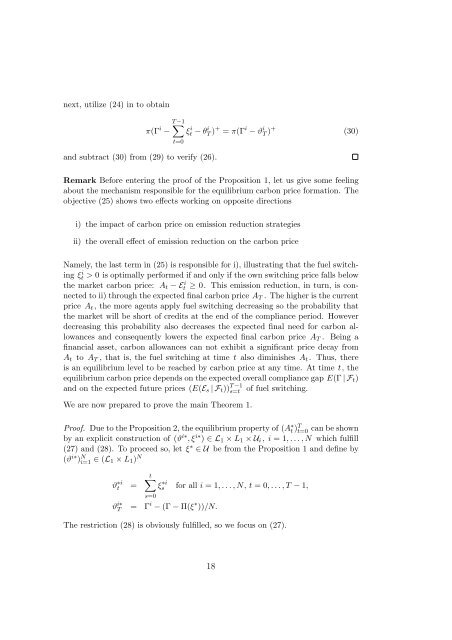
next, utilize (24) in <strong>to</strong> obtain<br />
T∑<br />
−1<br />
π(Γ i − ξt i − θT i ) + = π(Γ i − ϑ i T ) + (30)<br />
t=0<br />
and subtract (30) from (29) <strong>to</strong> verify (26).<br />
Remark Before entering the proof of the Proposition 1, let us give some feeling<br />
about the mechanism responsible for the equilibrium <strong>carbon</strong> <strong>price</strong> formation. The<br />
objective (25) shows two effects working on opposite directions<br />
i) the impact of <strong>carbon</strong> <strong>price</strong> on emission reduction strategies<br />
ii) the overall effect of emission reduction on the <strong>carbon</strong> <strong>price</strong><br />
Namely, the last term in (25) is responsible for i), illustrating that the fuel switching<br />
ξt i > 0 is optimally performed if and only if the own switching <strong>price</strong> falls below<br />
the market <strong>carbon</strong> <strong>price</strong>: A t − Et i ≥ 0. This emission reduction, in turn, is connected<br />
<strong>to</strong> ii) through the expected final <strong>carbon</strong> <strong>price</strong> A T . The higher is the current<br />
<strong>price</strong> A t , the more agents apply fuel switching decreasing so the probability that<br />
the market will be short of credits at the end of the compliance period. However<br />
decreasing this probability also decreases the expected final need for <strong>carbon</strong> allowances<br />
and consequently lowers the expected final <strong>carbon</strong> <strong>price</strong> A T . Being a<br />
financial asset, <strong>carbon</strong> allowances can not exhibit a significant <strong>price</strong> decay from<br />
A t <strong>to</strong> A T , that is, the fuel switching at time t also diminishes A t . Thus, there<br />
is an equilibrium level <strong>to</strong> be reached by <strong>carbon</strong> <strong>price</strong> at any time. At time t, the<br />
equilibrium <strong>carbon</strong> <strong>price</strong> depends on the expected overall compliance gap E(Γ | F t )<br />
and on the expected future <strong>price</strong>s (E(E s | F t )) T s=t<br />
−1 of fuel switching.<br />
We are now prepared <strong>to</strong> prove the main Theorem 1.<br />
Proof. Due <strong>to</strong> the Proposition 2, the equilibrium property of (A ∗ t ) T t=0 can be shown<br />
by an explicit construction of (ϑ i∗ , ξ i∗ ) ∈ L 1 × L 1 × U i , i = 1, . . . , N which fulfill<br />
(27) and (28). To proceed so, let ξ ∗ ∈ U be from the Proposition 1 and define by<br />
(ϑ i∗ ) N i=1 ∈ (L 1 × L 1 ) N<br />
ϑ ∗i<br />
t =<br />
t∑<br />
s=0<br />
ξ ∗i<br />
s for all i = 1, . . . , N, t = 0, . . . , T − 1,<br />
ϑ i∗<br />
T = Γ i − (Γ − Π(ξ ∗ ))/N.<br />
The restriction (28) is obviously fulfilled, so we focus on (27).<br />
18


