A quantitative approach to carbon price risk modeling - CiteSeerX

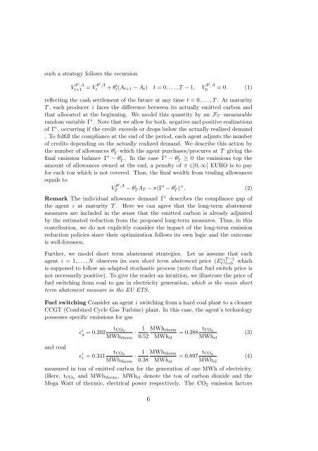
such a strategy follows the recursion
V θi ,A
t+1 = V θi ,A
t + θ i t(A t+1 − A t ) t = 0, . . . , T − 1, V θi ,A
0 = 0 (1)
reflecting the cash settlement of the future at any time t = 0, . . . , T . At maturity
T , each producer i faces the difference between its actually emitted carbon and
that allocated at the beginning. We model this quantity by an F T –measurable
random variable Γ i . Note that we allow for both, negative and positive realizations
of Γ i , occurring if the credit exceeds or drops below the actually realized demand
. To fulfill the compliance at the end of the period, each agent adjusts the number
of credits depending on the actually realized demand. We describe this action by
the number of allowances θT
i which the agent purchases/procures at T giving the
final emission balance Γ i − θT i . In the case Γi − θT
i ≥ 0 the emissions top the
amount of allowances owned at the end, a penalty of π ∈]0, ∞[ EURO is to pay
for each ton which is not covered. Thus, the final wealth from trading allowances
equals to
V θi ,A
T
− θT i A T − π(Γ i − θT i ) + . (2)
Remark The individual allowance demand Γ i describes the compliance gap of
the agent i at maturity T . Here we can agree that the long-term abatement
measures are included in the sense that the emitted carbon is already adjusted
by the estimated reduction from the proposed long-term measures. Thus, in this
contribution, we do not explicitly consider the impact of the long-term emission
reduction policies since their optimization follows its own logic and the outcome
is well-foreseen.
Further, we model short term abatement strategies. Let us assume that each
agent i = 1, . . . , N observes its own short term abatement price (Et) i T t=0 −1 which
is supposed to follow an adapted stochastic process (note that fuel switch price is
not necessarily positive). To give the reader an intuition, we illustrate the price of
fuel switching from coal to gas in electricity generation, which is the main short
term abatement measure in the EU ETS.
Fuel switching Consider an agent i switching from a hard coal plant to a cleaner
CCGT (Combined Cycle Gas Turbine) plant. In this case, the agent’s technology
possesses specific emissions for gas
and coal
e i t CO2 1 MWh therm
g = 0.202
·
= 0.388 t CO 2
(3)
MWh therm 0.52 MWh el MWh el
e i t CO2 1 MWh therm
c = 0.341
·
= 0.897 t CO 2
(4)
MWh therm 0.38 MWh el MWh el
measured in ton of emitted carbon for the generation of one MWh of electricity.
(Here, t CO2 and MWh therm , MWh el denote the ton of carbon dioxide and the
Mega Watt of thermic, electrical power respectively. The CO 2 emission factors
6