A quantitative approach to carbon price risk modeling - CiteSeerX

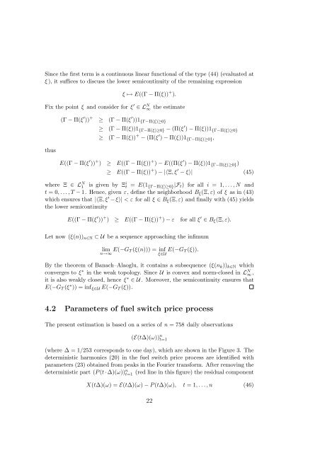
Since the first term is a continuous linear functional of the type (44) (evaluated at
ξ ), it suffices to discuss the lower semicontinuity of the remaining expression
ξ ↦→ E((Γ − Π(ξ)) + ).
Fix the point ξ and consider for ξ ′ ∈ L N ∞ the estimate
thus
(Γ − Π(ξ ′ )) + ≥ (Γ − Π(ξ ′ ))1 {Γ−Π(ξ)≥0}
≥ (Γ − Π(ξ))1 {Γ−Π(ξ)≥0} − (Π(ξ ′ ) − Π(ξ))1 {Γ−Π(ξ)≥0}
≥ (Γ − Π(ξ)) + − (Π(ξ ′ ) − Π(ξ))1 {Γ−Π(ξ)≥0} ,
E((Γ − Π(ξ ′ )) + ) ≥ E((Γ − Π(ξ)) + ) − E((Π(ξ ′ ) − Π(ξ))1 {Γ−Π(ξ)≥0} )
≥ E((Γ − Π(ξ)) + ) − |〈Ξ, ξ ′ − ξ〉| (45)
where Ξ ∈ L N 1 is given by Ξ i t = E(1 {Γ−Π(ξ)≥0} |F t ) for all i = 1, . . . , N and
t = 0, . . . , T − 1. Hence, given ε, define the neighborhood B ξ (Ξ, ε) of ξ as in (43)
which ensures that |〈Ξ, ξ ′ − ξ〉| < ε for all ξ ∈ B ξ (Ξ, ε) and finally with (45) yields
the lower semicontinuity
E((Γ − Π(ξ ′ )) + ) ≥ E((Γ − Π(ξ)) + ) − ε for all ξ ′ ∈ B ξ (Ξ, ε).
Let now (ξ(n)) n∈N ⊂ U be a sequence approaching the infimum
lim E(−G T (ξ(n))) = inf E(−G T (ξ)).
n→∞ ξ∈U
By the theorem of Banach–Alaoglu, it contains a subsequence (ξ(n k )) k∈N which
converges to ξ ∗ in the weak topology. Since U is convex and norm-closed in L N ∞ ,
it is also weakly closed, hence ξ ∗ ∈ U . Moreover, the semicontinuity ensures that
E(−G T (ξ ∗ )) = inf ξ∈U E(−G T (ξ)).
4.2 Parameters of fuel switch price process
The present estimation is based on a series of n = 758 daily observations
(E(t∆)(ω)) n t=1
(where ∆ = 1/253 corresponds to one day), which are shown in the Figure 3. The
deterministic harmonics (20) in the fuel switch price process are identified with
parameters (23) obtained from peaks in the Fourier transform. After removing the
deterministic part (P (t · ∆)(ω)) n t=1 (red line in this figure) the residual component
X(t∆)(ω) = E(t∆)(ω) − P (t∆)(ω), t = 1, . . . , n (46)
22