A quantitative approach to carbon price risk modeling - CiteSeerX

More documents

Recommendations

Info

Since the first term is a continuous linear functional of the type (44) (evaluated at ξ ), it suffices to discuss the lower semicontinuity of the remaining expression ξ ↦→ E((Γ − Π(ξ)) + ). Fix the point ξ and consider for ξ ′ ∈ L N ∞ the estimate thus (Γ − Π(ξ ′ )) + ≥ (Γ − Π(ξ ′ ))1 {Γ−Π(ξ)≥0} ≥ (Γ − Π(ξ))1 {Γ−Π(ξ)≥0} − (Π(ξ ′ ) − Π(ξ))1 {Γ−Π(ξ)≥0} ≥ (Γ − Π(ξ)) + − (Π(ξ ′ ) − Π(ξ))1 {Γ−Π(ξ)≥0} , E((Γ − Π(ξ ′ )) + ) ≥ E((Γ − Π(ξ)) + ) − E((Π(ξ ′ ) − Π(ξ))1 {Γ−Π(ξ)≥0} ) ≥ E((Γ − Π(ξ)) + ) − |〈Ξ, ξ ′ − ξ〉| (45) where Ξ ∈ L N 1 is given by Ξ i t = E(1 {Γ−Π(ξ)≥0} |F t ) for all i = 1, . . . , N and t = 0, . . . , T − 1. Hence, given ε, define the neighborhood B ξ (Ξ, ε) of ξ as in (43) which ensures that |〈Ξ, ξ ′ − ξ〉| < ε for all ξ ∈ B ξ (Ξ, ε) and finally with (45) yields the lower semicontinuity E((Γ − Π(ξ ′ )) + ) ≥ E((Γ − Π(ξ)) + ) − ε for all ξ ′ ∈ B ξ (Ξ, ε). Let now (ξ(n)) n∈N ⊂ U be a sequence approaching the infimum lim E(−G T (ξ(n))) = inf E(−G T (ξ)). n→∞ ξ∈U By the theorem of Banach–Alaoglu, it contains a subsequence (ξ(n k )) k∈N which converges to ξ ∗ in the weak topology. Since U is convex and norm-closed in L N ∞ , it is also weakly closed, hence ξ ∗ ∈ U . Moreover, the semicontinuity ensures that E(−G T (ξ ∗ )) = inf ξ∈U E(−G T (ξ)). 4.2 Parameters of fuel switch price process The present estimation is based on a series of n = 758 daily observations (E(t∆)(ω)) n t=1 (where ∆ = 1/253 corresponds to one day), which are shown in the Figure 3. The deterministic harmonics (20) in the fuel switch price process are identified with parameters (23) obtained from peaks in the Fourier transform. After removing the deterministic part (P (t · ∆)(ω)) n t=1 (red line in this figure) the residual component X(t∆)(ω) = E(t∆)(ω) − P (t∆)(ω), t = 1, . . . , n (46) 22
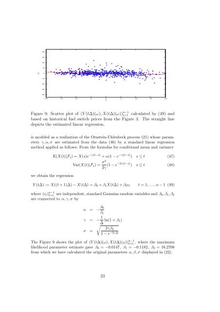
40 30 20 10 ∆X 0 -10 -20 -30 -40 -20 -15 -10 -5 0 5 10 15 20 X Figure 9: Scatter plot of (Y (t∆)(ω), X(t∆)(ω)) n−1 t=1 calculated by (49) and based on historical fuel switch prices from the Figure 3. The straight line depicts the estimated linear regression. is modeled as a realization of the Ornstein-Uhlenbeck process (21) whose parameters γ, α, σ are estimated from the data (46) by a standard linear regression method applied as follows: From the formulas for conditional mean and variance we obtain the regression E(X(t)|F s ) = X(s)e −γ(t−s) + α(1 − e −γ(t−s) ) s ≤ t (47) Var(X(t)|F s ) = σ2 2γ (1 − e−2γ(t−s) ) s ≤ t (48) Y (t∆) := X((t + 1)∆) − X(t∆) = β 0 + β 1 X(t∆) + β 2 ɛ t t = 1, . . . , n − 1 (49) where (ɛ t ) n−1 t=1 are independent, standard Gaussian random variables and β 0, β 1 , β 2 are connected to α, γ, σ by α = − β 0 β 1 γ = − 1 ∆ ln(1 + β 1) √ 2γβ2 σ = 1 − e −2γ∆ The Figure 9 shows the plot of (Y (t∆)(ω), X(t∆)(ω)) t=1 n−1 , where the maximum likelihood parameter estimate gave β 0 = −0.0147, β 1 = −0.1182, β 2 = 16.2708 from which we have calculated the original parameters α, β, σ displayed in (22). 23
Page 1 and 2: A quantitative approach to carbon p
Page 3 and 4: • for the IET mechanism, these cr
Page 5 and 6: and JI- projects. On the contrary,
Page 7 and 8: are default values provided by the
Page 9 and 10: With these notations, the equilibri
Page 11 and 12: period 2008-2012 and, more importan
Page 13 and 14: in Mega tons of carbon dioxide. Num
Page 15 and 16: Let us summarize our findings. The
Page 17 and 18: Given the fuel switching policy (ξ
Page 19 and 20: For ϑ ∈ (L 1 × L 1 ) N , ξ ∈
Page 21: which with (40) implies that the fo
Page 25: [15] J. Seifert, M. Uhrig-Homburg,

A quantitative approach to carbon price risk modeling - CiteSeerX

Create successful ePaper yourself

Delete template?

Save as template?