A quantitative approach to carbon price risk modeling - CiteSeerX

More documents

Recommendations

Info

such a strategy follows the recursion V θi ,A t+1 = V θi ,A t + θ i t(A t+1 − A t ) t = 0, . . . , T − 1, V θi ,A 0 = 0 (1) reflecting the cash settlement of the future at any time t = 0, . . . , T . At maturity T , each producer i faces the difference between its actually emitted carbon and that allocated at the beginning. We model this quantity by an F T –measurable random variable Γ i . Note that we allow for both, negative and positive realizations of Γ i , occurring if the credit exceeds or drops below the actually realized demand . To fulfill the compliance at the end of the period, each agent adjusts the number of credits depending on the actually realized demand. We describe this action by the number of allowances θT i which the agent purchases/procures at T giving the final emission balance Γ i − θT i . In the case Γi − θT i ≥ 0 the emissions top the amount of allowances owned at the end, a penalty of π ∈]0, ∞[ EURO is to pay for each ton which is not covered. Thus, the final wealth from trading allowances equals to V θi ,A T − θT i A T − π(Γ i − θT i ) + . (2) Remark The individual allowance demand Γ i describes the compliance gap of the agent i at maturity T . Here we can agree that the long-term abatement measures are included in the sense that the emitted carbon is already adjusted by the estimated reduction from the proposed long-term measures. Thus, in this contribution, we do not explicitly consider the impact of the long-term emission reduction policies since their optimization follows its own logic and the outcome is well-foreseen. Further, we model short term abatement strategies. Let us assume that each agent i = 1, . . . , N observes its own short term abatement price (Et) i T t=0 −1 which is supposed to follow an adapted stochastic process (note that fuel switch price is not necessarily positive). To give the reader an intuition, we illustrate the price of fuel switching from coal to gas in electricity generation, which is the main short term abatement measure in the EU ETS. Fuel switching Consider an agent i switching from a hard coal plant to a cleaner CCGT (Combined Cycle Gas Turbine) plant. In this case, the agent’s technology possesses specific emissions for gas and coal e i t CO2 1 MWh therm g = 0.202 · = 0.388 t CO 2 (3) MWh therm 0.52 MWh el MWh el e i t CO2 1 MWh therm c = 0.341 · = 0.897 t CO 2 (4) MWh therm 0.38 MWh el MWh el measured in ton of emitted carbon for the generation of one MWh of electricity. (Here, t CO2 and MWh therm , MWh el denote the ton of carbon dioxide and the Mega Watt of thermic, electrical power respectively. The CO 2 emission factors 6
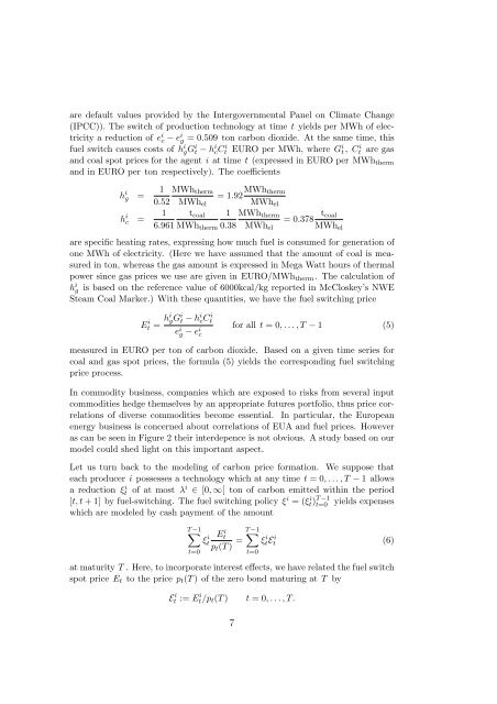
are default values provided by the Intergovernmental Panel on Climate Change (IPCC)). The switch of production technology at time t yields per MWh of electricity a reduction of e i c − e i g = 0.509 ton carbon dioxide. At the same time, this fuel switch causes costs of h i gG i t − h i cC i t EURO per MWh, where G i t , C i t are gas and coal spot prices for the agent i at time t (expressed in EURO per MWh therm and in EURO per ton respectively). The coefficients h i g = h i c = MWh therm 1 = 1.92 MWh therm 0.52 MWh el MWh el 1 t coal 1 MWh therm = 0.378 t coal 6.961 MWh therm 0.38 MWh el MWh el are specific heating rates, expressing how much fuel is consumed for generation of one MWh of electricity. (Here we have assumed that the amount of coal is measured in ton, whereas the gas amount is expressed in Mega Watt hours of thermal power since gas prices we use are given in EURO/MWh therm . The calculation of h i g is based on the reference value of 6000kcal/kg reported in McCloskey’s NWE Steam Coal Marker.) With these quantities, we have the fuel switching price E i t = hi gG i t − h i cC i t e i g − e i c for all t = 0, . . . , T − 1 (5) measured in EURO per ton of carbon dioxide. Based on a given time series for coal and gas spot prices, the formula (5) yields the corresponding fuel switching price process. In commodity business, companies which are exposed to risks from several input commodities hedge themselves by an appropriate futures portfolio, thus price correlations of diverse commodities become essential. In particular, the European energy business is concerned about correlations of EUA and fuel prices. However as can be seen in Figure 2 their interdepence is not obvious. A study based on our model could shed light on this important aspect. Let us turn back to the modeling of carbon price formation. We suppose that each producer i possesses a technology which at any time t = 0, . . . , T − 1 allows a reduction ξt i of at most λ i ∈ [0, ∞[ ton of carbon emitted within the period [t, t + 1] by fuel-switching. The fuel switching policy ξ i = (ξt) i T t=0 −1 yields expenses which are modeled by cash payment of the amount ∑ T −1 ξt i t=0 Et i T −1 p t (T ) = ∑ ξtE i t i (6) at maturity T . Here, to incorporate interest effects, we have related the fuel switch spot price E t to the price p t (T ) of the zero bond maturing at T by t=0 E i t := E i t/p t (T ) t = 0, . . . , T. 7
Page 1 and 2: A quantitative approach to carbon p
Page 3 and 4: • for the IET mechanism, these cr
Page 5: and JI- projects. On the contrary,
Page 9 and 10: With these notations, the equilibri
Page 11 and 12: period 2008-2012 and, more importan
Page 13 and 14: in Mega tons of carbon dioxide. Num
Page 15 and 16: Let us summarize our findings. The
Page 17 and 18: Given the fuel switching policy (ξ
Page 19 and 20: For ϑ ∈ (L 1 × L 1 ) N , ξ ∈
Page 21 and 22: which with (40) implies that the fo
Page 23 and 24: 40 30 20 10 ∆X 0 -10 -20 -30 -40
Page 25: [15] J. Seifert, M. Uhrig-Homburg,

A quantitative approach to carbon price risk modeling - CiteSeerX

Create successful ePaper yourself

Delete template?

Save as template?