Estimation in Financial Models - RiskLab
Estimation in Financial Models - RiskLab
Estimation in Financial Models - RiskLab
You also want an ePaper? Increase the reach of your titles
YUMPU automatically turns print PDFs into web optimized ePapers that Google loves.
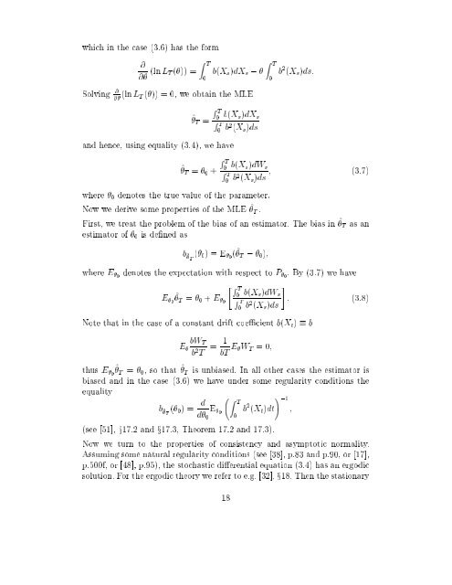
which <strong>in</strong> the case (3.6) has the form<br />
@<br />
@ (ln L T ()) =<br />
Z T<br />
0<br />
b(X s )dX s , <br />
Solv<strong>in</strong>g @ @ (ln L T ()) = 0, we obta<strong>in</strong> the MLE<br />
Z T<br />
0<br />
b 2 (X s )ds:<br />
^ T =<br />
R T<br />
R<br />
0<br />
T<br />
0<br />
b(X s )dX s<br />
b 2 (X s )ds<br />
and hence, us<strong>in</strong>g equality (3.4), we have<br />
^ T = 0 +<br />
where 0 denotes the true value of the parameter.<br />
Now we derive some properties of the MLE ^ T .<br />
R T<br />
0<br />
b(X s )dW R<br />
s<br />
T<br />
0<br />
b 2 (X s )ds ; (3.7)<br />
First, we treat the problem of the bias of an estimator. The bias <strong>in</strong> ^ T as an<br />
estimator of 0 is dened as<br />
b^ T<br />
( 0 )=E 0 (^ T , 0 );<br />
where E 0<br />
denotes the expectation with respect to P 0 . By (3.7) we have<br />
"R T<br />
#<br />
0<br />
b(X s )dW s<br />
E 0<br />
^T = 0 + E 0 : (3.8)<br />
b 2 (X s )ds<br />
R T<br />
0<br />
Note that <strong>in</strong> the case of a constant drift coecient b(X t ) b<br />
E <br />
bW T<br />
b 2 T = 1<br />
bT E W T =0;<br />
thus E 0<br />
^T = 0 , so that ^ T is unbiased. In all other cases the estimator is<br />
biased and <strong>in</strong> the case (3.6) we have under some regularity conditions the<br />
equality<br />
b^ T<br />
( 0 )=<br />
d Z T<br />
,1<br />
E 0 b 2 (X t )dt!<br />
;<br />
d 0 0<br />
(see [51], x17.2 and x17.3, Theorem 17.2 and 17.3).<br />
Now we turn to the properties of consistency and asymptotic normality.<br />
Assum<strong>in</strong>g some natural regularity conditions (see [38], p.83 and p.90, or [17],<br />
p.500f, or [48], p.95), the stochastic dierential equation (3.4) has an ergodic<br />
solution. For the ergodic theory we refer to e.g. [32], x18. Then the stationary<br />
18


