Estimation in Financial Models - RiskLab

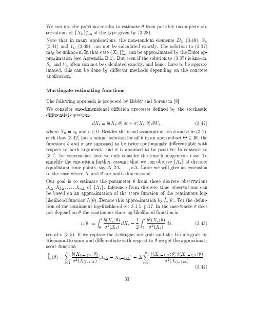
We can use the previous results to estimate from possibly incomplete observations
of fX ti g n i=0
of the type given by (3.28).
Note that in many applications, the non-random elements D ti (3.40), S ti
(3.41) and V ti (3.39), can not be calculated exactly. The solution to (3.37)
may be unknown. In that case fX ti g n i=0
can be approximated by the Euler approximation
(see Appendix B.1). But even if the solution to (3.37) is known,
S ti and V ti often can not be calculated exactly, and hence have to be approximated;
this can be done by dierent methods depending on the concrete
application.
Martingale estimating functions
The following approach is proposed by Bibby and Srensen [8].
We consider one-dimensional diusion processes dened by the stochastic
dierential equations
dX t = b(X t ; ) dt + (X t ; ) dW t ; (3.42)
where X 0 = x 0 and t 0. Besides the usual assumptions on b and in (3.1),
such that (3.42) has a unique solution for all in an open subset IR, the
functions b and are supposed to be twice continuously dierentiable with
respect to both arguments and is assumed to be positive. In contrast to
(3.1), for convenience here we only consider the time-homogeneous case. To
simplify the exposition further, assume that we can observe fX t g at discrete
equidistant time points, say ; 2;:::;n. Later we will give an extension
to the case where X and are multi-dimensional.
Our goal is to estimate the parameter from these discrete observations
X ;X 2 ;:::;X n of fX t g. Inference from discrete time observations can
be based on an approximation of the score function of the continuous loglikelihood
function l t (). Denote this approximation by ~ _ ln (). For the denition
of the continuous log-likelihood see 3.1.1, p.17. In the case where does
not depend on the continuous time log-likelihood function is
l t () =
Z t
0
b(X s ; )
2 (X s ) dX s , 1 2
Z t
0
b 2 (X s ; )
2 (X s )
ds; (3.43)
see also (3.5). If we replace the Lebesgue integrals and the It^o integrals by
Riemann-It^o sums and dierentiate with respect to we get the approximate
score function
nX _b(X (i,1) ; )
nX
_~l n () =
i=1
2 (X (i,1) ) (X b(X (i,1) ; ) b(X
i , X (i,1) ) ,
_ (i,1) ; )
:
i=1
2 (X (i,1) )
(3.44)
33