Estimation in Financial Models - RiskLab

where X 0 = 0 and t 0, the log-likelihood function l n () is unknown. The
approximate log-likelihood functions (l n;N ()) 1 N=1
can be used to estimate ,
because (3.25) has a weak solution for all x 0 and for all >0 which is unique
in law and (A4) is satised for all >0.
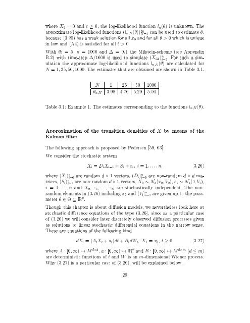
With 0 = 5, n = 1000 and = 0:1 the Milstein-scheme (see Appendix
B.2) with time-step =1000 is used to simulate (X i ) n i=0. For such a simulation
the approximate log-likelihood functions l n;N () are calculated for
N =1; 25; 50; 1000. The estimates that are obtained are shown in Table 3.1.
N 1 25 50 1000
^ n;N 3.98 4.76 5.20 5.04
Table 3.1: Example 1. The estimates corresponding to the functions l n;N ().
Approximation of the transition densities of X by means of the
Kalman lter
The following approach is proposed by Pedersen [59, 63].
We consider the stochastic system
X i = D i X i,1 + S i + " i ; i =1;:::;n; (3.26)
where (X i ) n i=0
are random d 1 vectors, (D i ) n i=0
are non-random d d matrices,
(S i ) n i=1
are non-random d 1vectors, X 0 N d (x 0 ;V 0 ), " i N d (0;V i ),
i = 1;:::;n and X 0 , " 1 ;:::, " n are stochastically independent. The nonrandom
elements in (3.26) including x 0 and (V i ) n i=0
are given up to the parameter
2 IR p .
Though this chapter is about diusion models, we nevertheless look here at
stochastic dierence equations of the type (3.26), since as a particular case
of (3.26) we will consider later discretely observed diusion processes given
as solutions to linear stochastic dierential equations in the narrow sense.
These are equations of the following kind
dX t =(A t X t + a t )dt + B t dW t ; X 0 = x 0 ; t 0; (3.27)
where A :[0; 1) 7! M dd , a :[0; 1) 7! IR d and B :[0; 1) 7! M dm (d m)
are deterministic functions of t and W is an m-dimensional Wiener process.
Why (3.27) is a particular case of (3.26), will be explained below.
29