advances in numerical modeling of manufacturing processes

TRANS. INDIAN INST. MET., VOL. 57, NO. 4, AUGUST 2004
objective of eliminating end cracking in the extruded
shafts, it is necessary to contain the maximum
circumferential stress (
) and the maximum axial
stress ( z
) below the fracture strength of the material
in circumferential tension and uniaxial tension,
respectively (i.e.,
< 107.5 ksi and z
< 98 ksi).
Minimize:
= (136.19) – (138.74*a) + (0.48*b) +
(90.61*c) + (6.59*d) – (1022.8*e) +
(43.33*a 2 ) – (1.39*d 2 ) + (496.06*e 2 ) +
(7.5*a*d) + (381.23*a*e) + (90.22*d*e)
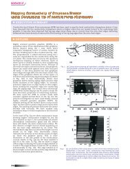
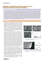
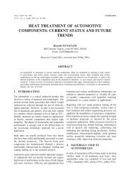
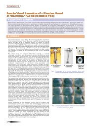
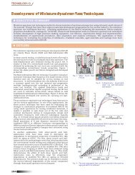
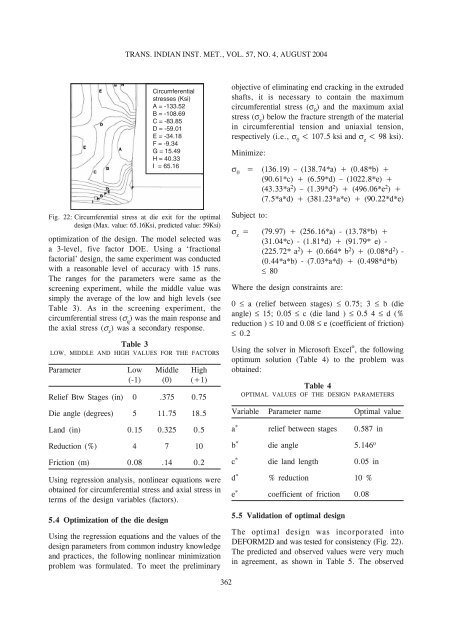
Fig. 22: Circumferential stress at die exit for the optimal
design (Max. value: 65.16Ksi, predicted value: 59Ksi)
optimization of the design. The model selected was
a 3-level, five factor DOE. Using a ‘fractional
factorial’ design, the same experiment was conducted
with a reasonable level of accuracy with 15 runs.
The ranges for the parameters were same as the
screening experiment, while the middle value was
simply the average of the low and high levels (see
Table 3). As in the screening experiment, the
circumferential stress ( q
) was the main response and
the axial stress ( z
) was a secondary response.
Table 3
LOW, MIDDLE AND HIGH VALUES FOR THE FACTORS
Parameter Low Middle High
(-1) (0) (+1)
Relief Btw Stages (in) 0 .375 0.75
Die angle (degrees) 5 11.75 18.5
Land (in) 0.15 0.325 0.5
Reduction (%) 4 7 10
Friction (m) 0.08 .14 0.2
Using regression analysis, nonlinear equations were
obtained for circumferential stress and axial stress in
terms of the design variables (factors).
5.4 Optimization of the die design
Using the regression equations and the values of the
design parameters from common industry knowledge
and practices, the following nonlinear minimization
problem was formulated. To meet the preliminary
Subject to:
z
= (79.97) + (256.16*a) - (13.78*b) +
(31.04*c) - (1.81*d) + (91.79* e) -
(225.72* a 2 ) + (0.664* b 2 ) + (0.08*d 2 ) -
(0.44*a*b) - (7.03*a*d) + (0.498*d*b)
80
Where the design constraints are:
0 a (relief between stages) 0.75; 3 b (die
angle) 15; 0.05 c (die land ) 0.5 4 d (%
reduction ) 10 and 0.08 e (coefficient of friction)
0.2
Using the solver in Microsoft Excel ® , the following
optimum solution (Table 4) to the problem was
obtained:
Table 4
OPTIMAL VALUES OF THE DESIGN PARAMETERS
Variable Parameter name Optimal value
a * relief between stages 0.587 in
b * die angle 5.146 o
c * die land length 0.05 in
d * % reduction 10 %
e * coefficient of friction 0.08
5.5 Validation of optimal design
The optimal design was incorporated into
DEFORM2D and was tested for consistency (Fig. 22).
The predicted and observed values were very much
in agreement, as shown in Table 5. The observed
362