Saddleback Journal of Biology - Saddleback College

Saddleback 

Journal of Biology 

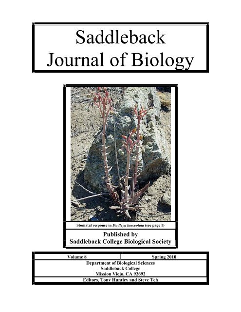
Stomatal response in Dudleya lanceolata (see page 1) 

Published by 

Saddleback College Biological Society 

Volume 8 Spring 2010 

Department of Biological Sciences 

Saddleback College 

Mission Viejo, CA 92692 

Editors, Tony Huntley and Steve Teh

TABLE OF CONTENTS 

Peer Reviewed Manuscripts from the Biology 3B Class 

Spring 2010 

Author(s) Title Page 

JenniferOberholtzer& Dark Stomatal Response and Carbon Dioxide Levels in 1 

Amanda Swanson 

Dudleya lanceolata at Various Humidities 

Khoa Tran The Effect of Sodium Chloride Concentration on the Growth 4 

of Bread Mold 

Linda Mahoney Effect of Artificial Concentrated Feeding Area Resource 7 

& 

Kathleen Kuechler 

Depression on the Territoriality of the Anna Hummingbird 

(Calypte anna) 

Daria Cubberley Effect of Various Salinities of Water on Osmoregulation in 

Green Shore Crab 

12 

Kenneth Tupper 

& 

Cole Querry 

Ryan Palhidai 

& 

Chelsea Santos 

Dustin Cheverier & 

Edgar Gomez 

Eric Rueda 

Scott Lilly 

& 

Jordan Meek 

Chelsea Lindwall 

Sherwin Jenabian 

Brian W Capen 

& 

Paige H Taylor 

The effect of the menstrual cycle on sexual selection in 

Homo sapiens based on olfactory cues 

The Effect of an Injected Glutamine Load on Time to 

Exhaustion in Western Fence Lizards 

(Sceloporus occidentalis 

Garlic (Allium sativum) as an Antibacterial Component 

against Salmonella in Beef 

The Effect of essential oil of Oregano (Origanum vulgare) 

on the in vitro growth of the bacteria Escherichia coli, 

Salmonella typhimurium, and Staphylococcus aureus 

Growth Inhibition of Escherichia coli. by Essential Oils of 

Rosemary (Rosmarinus officinalis) and Lavender (Lavandula 

augustifolia) 

Humerus to Radius Ratio and Its Effect on Stride Length in 

Canis familiaris 

Time of Day Effects on The Assembly Call on The 

American Crow(Corvus americanus) 

The Effect of Near Freezing Temperatures on Blood Glucose 

Levels in Hyla regilla Collected in Coastal Southern 

California 

Sophia Iribarren Effect of pH on vinegar eel (Turbatrix aceti) 45 

Sara Rose A Comparison of the Effectiveness of Time of Day and 47 

& 

Michelle Garcia 

Lures on Largemouth Bass (Micropterus salmoides) in Lake 

Mission Viejo 

Kasra Sadjadi & Comparison of Vital Lung Capacity between Smokers and 51 

Cassra Minai 

Non-Smokers 

Paul Nix Effect of Caffeine on the Metabolic and Respiration of the 

Common Goldfish 

53 

15 

19 

22 

29 

32 

35 

37 

40 

ii 

Saddleback Journal of Biology 

Vol. 8, Spring 2010


Peer Reviewed Manuscripts from the Biology 3B Class 

Fall 2009 


Stephanie Melton & Effect of Blood Donation Frequency and Gender on 57 

Jessica Ochoa 

Physiological Response to Blood Loss 

Michael Wan Knockdown and Effect of Lactational Hormones on CTR-1 64 

and Cerulopasmin 

Timothy Schang & Recovery and Growth of Vegetation Pre and Post Wildland 71 

Vanessa Haber 

Fire in the Chaparral of Southern California 

Jennifer Doncost & The Effect of Altitude on the Metabolic Rate in Sceloporus 75 

Andrew Naillon 

occidentalis 

Rose Park & The Effects of Temperature on Rates of Metamorphosis in 80 

Laura Chan 

Vanessa cardui 

Laura Powell & Effects of Tobacco Use on the Vital Lung Capacity of 85 

Nicole Mills 

Healthy Male Students 

Brett Niles & The Effect of Green Tea and Deionized Water on the Growth 87 

Carlin Harkness Rate and Chlorophyll Concentration of Catharanthus roseus 

Chelsea Roche & The Difference in Metabolic Rate of Quail Eggs During 91 

Frank Leon 

Incubation 

Sheena Forsberg & The Impact of Organic Soil on Growth Rate and Average Yield 94 

Christopher Thompson 

of Wisconsin Fast Plants 

Hamidreza Hoveida& The Preference of Different Colored Seeds by Birds in 97 

Sean Kouyoumdjian 

Laguna Niguel, California 

Sara Rose & Comparison of Forced Vital Capacity among Trumpet 100 

Kristianne Salcines 

Instrumentalists and Water Polo Players 

Brennan Buchan & Comparison of Water Versus Gatorade Hydration on 103 

Kristin Fiore 

VO2max and Maximal Exercise Time in Athletes 

Sean Parsa & 

The Effects of Creatine Monohydrate on 

106 

Heeva Ghane 

White Mice (Mus musculus) 

Niku Borujerdpur, The Effect of Cool down Laps on Lactate Recovery Rates In 109 

Nathan Nguyen & 

Kristina Nikkhah 

Male Water Polo 

Anahita A. Ariarad & The Effects of Combined Rider and Tack Weight on the 112 

Allison S. Lindsay Lactic Acid Production in the Horse at Three Different Gaits 

Alvin Jogasuria & Efficacy of Bicarbonate containing Chewing Gum on the 116 

Eric Taysom 

Salivary Flow and pH in Humans 

Shirin Moftakhar & The Effects of Cranberry Juice on Urinary Tract Infection 120 

Assal Parsa 

Causing Bacteria, Echerichia coli 

Yousif Astarabadi & The Effect of Aerobic Exercise on Human Short-Term 123 

Hannah Ogren 

Memory 

Beau Gentry & Comparison of the Soluble Phosphorous in Urban and Rural 126 

Patrick Schafer 

Sarai Finks & 

Kazuhiro Sabet 

Aquatic Environments 

Response of Staphylococcus aureus to acetylsalicylate 

challenge while in the presence of Notatum penicillium 

iii 


Vol. 8, Spring 2010 

128

Kim Chené & 

Water Quality at Doheny State Beach 132 

Brittany Harding 

Jessica Garcia & The Density of Marine Organisms in Intertidal Ecosystems 135 

Jackie Olvera 

Mohammad Dadkhah The Comparison of Strawberry Extract on the growth of two 138 

& 

Amin Najmabadi 

Different Gram-negative Bacteria 

Alex Tran & The Effect of Shipping Activity on Growth of Lottia 141 

Eric Haffner 

strigatella and Tegula funebralis 

Jonathon So Comparative Sterilization of Escherichia coli 145 

Krystina Jarema 

The Effects of Temperature on Succinic Acid 

Dehydrogenase activity in Cold and Warm Adapted Fish 

147 

Biology 3A abstracts for papers presented at the 8 th Annual Biology 3A/3B 

Scientific Meeting (Spring 2010) 

The meeting organizers do not assume responsibility for any inconsistencies in quality or 

errors in abstract information. Abstracts are in numerical order according to the abstract 

number assigned to each presentation. Authorless abstracts appear at the end of all the 

abstracts, including non-submitted abstracts, if any. Abstracts begin on page 151. 


Biology 3A Abstracts 

Spring 2010 


Emily Rounds & THE EFFECT OF CALCIUM ION CONCENTRATION ON 151 

Gianne Acosta OSMOREGULATION IN GOLDFISH (Carassius auratus). 

Crystal Shum RECOVERY RATE OF LACTIC ACID SHOCK WHEN 151 

& 

Scott Skaggs 

BUFFERED BY SODIUM BICARBONATE ON Sceloporus 

occidentalis 

Lawrence Hohman EFFECT OF HYDROCHLORIC ACID ON EXHAUSTION 151 

& William Whitlock POINT IN SCELOPORUS OCCIDENTALIS 

Seyed Pairawan & THE EFFECT OF STEVIA ON MOUSE WEIGHT 152 

Yumika Shimoda 

(Mus musculus) 

Richard Triggs & 

Adam Gordon 

EFFECT OF LIGHT WAVELENGTH ON METABOLIC 

RATES IN Gromphadorhina portentosa 

152 

Eden Perez 

& 

Sasha Jamshidi 

Phyllis Chong 

& 

Ida Jelveh 

A COMPARISON OF THE METABOLIC RATES IN 

MALE AND FEMALE MADAGASCAR HISSING 

COCKROACHES (Gromphadorhina portentosa) 

RELATIONSHIP BETWEEN THE ATTRACTIVENESS OF 

BODY ODOR TO BILATERAL FACIAL SYMMETRY IN 

MALE HUMANS 

iv 



152 

153


Angela C. Park & 

THE EFFECT OF VARIOUS SLOPES ON A 

153 

Michael A. Corrado SNOWBOARDERS (Homo sapiens) HEART RATE 

Neda Sanai THE ALLOMETRIC RELATIONSHIP DUE TO MASS 153 

& 

Austin Anderson 

SPECIFIC METABOLIC RATE OF MADAGASCAR 

HISSING COCKROACHES (Gromphadorhina portentosa) 

Jessica Dizon & PH LEVELS OF CRASSULA OVATA GROWN UNDER 154 

Shabnam Sadat 

RED LIGHT AND BLUE LIGHT 

Jasmine Singh & 

GROWTH OF MOLD (Penicillium notatum) 

154 

Donna Tehrani 

IN RESPSECT TO pH 

Charlie Paine & 

Kate Wang 

THE EFFECT OF HYDRATION ON BLOOD GLUCOSE 

LEVELS 

154 

Darren McAffee 

& 

Carly Purcell 

Tyler Finck & 

Matt Tolles 

Hannah Giclas & 

Khodayar Khatiblou 

Elizabeth Anderson 

& Dan Kim 

Andrew Tran & 

Nathan Famatigan 

Austin Arruda 

& 

Michael Bezer 

Pablo S. Kang & 

Grace Naddour 

Allison Le 

& 

Natalie Manzo 

Julian Galvis & 

Jay Cloyd 

Marissa R. Quijano 

& Parisa Karimian 

MOTILE RESPONSE OF MADAGASCAR HISSING 

COCKROACH GROMPHADORHINA PORTENTOSA TO 

PRESENCE OF NECROMONES 

METAL RETETION OF TIN AND IRON IN AN AQUATIC 

FRESHWATER PLANT (Elodea canadensis) 

THE EFFECT OF ELEVATION ON THE METABOLIC 

RATE OF MICE (Mus musculus) 

THE EFFECTS OF TEMPERATURE ON LACTATE 

DEHYDROGENASE OF GOLDFISH (Carassius auratus) 

AFFECT OF SALINITY ON THE PH OF A 

CRASSULACEAN ACID METABOLISM PLANT 

(Crassula ovata) 

THE EFFECT OF ALTITUDE CHANGE ON THE 

METABOLIC RATE OF THE WESTERN FENCE 

LIZARD, Sceloporus occidentalis 

WEIGHT SPECIFIC METABOLIC RATE IN ESTIVATING 

LAND SNAILS (Helix aspersa). 

THE EFFECT OF DIFFERENT TEMPERATURES ON 

THE CLOSING RATE OF VENUS FLYTRAPS 

(Dionaea muscipula) 

TEMPERATURE EFFECTS ON THE STOMATA OF 

DUDLEYA LANCEOLATA 

THE EFFECT OF LACCASE ENZYME EXTRACTED 

FROM TRAMETES VERSICOLOR ON POLYBISPHENOL- 

A EPICHLOROHYDRIN 

155 

155 

155 

156 

156 

156 

157 

157 

158 

158 

v 


Vol. 8, Spring 2010

Biology 3A abstracts for papers presented at the Annual Biology 3A 

Poster Presentation Scientific Meeting (Fall 2009) 

The meeting organizers do not assume responsibility for any inconsistencies in quality or 

errors in abstract information. Abstracts are in numerical order according to the abstract 

number assigned to each presentation. Authorless abstracts appear at the end of all the 

abstracts, including non-submitted abstracts, if any. Abstracts begin on page 159. 



Fall 2009 


M. Cole Miller & EFFECT OF CAFFEINE ON THE METABOLIC RATES OF 159 

Braden A. Altstatt 

MICE (Mus musculus) 

Setareh Amoozadeh THE USE OF EDGES IN VISUAL NAVIGATION BY THE 159 

ANTS (Tetramorium caespitum) 

Brian Atwood & THE EFFECTS OF PIRACETAM ON MAZE LEARNING IN 159 

Caroline Byeon 

MUS MUSCULUS 

Bernard Bouzari & AFFECTS OF VARYING PH LEVELS ON RADISH SEED 160 

Andia Safavi 

GERMINATION (Raphanus sativus) 

Dustin C. Cheverier & 

Edgar N. Gomez 

THE ANTIBACTERIAL PROPERTIES OF GARLIC (Allium 

sativum) ON BEEF AGAR 

160 

Kyle Crawford 

& 

Chris Medina 

Daria Cubberley 

& 

Arshan Ferdowsian 

Saman Hashemi 

Maral Iftekhary & 

Sophia Iribarren 

Casey R. Burgwald & 

Ronald T. Istrat 

Kathleen Kuechler & 

Lara Quintanar 

Rodrigo Moreno & 

Scott Lilly 

Jane H. Lim & 

Vy M. Nguyen 

Linda Mahoney & 

Sheeda Sanai 

Jennifer A.Oberholtzer 

&Amanda C. Swanson 

INTRASPECIFIC VARIATION IN RESISTANCE AND 

ADAPTATION TO DESICCATION AND CLIMATIC 

GRADIENTS IN THE PACIFIC BANANA SLUG (Ariolimax 

columbianus) 

CRUDE ONION (Allium cepa) JUICE SHOWS NO 

SIGNIFICANT ANTIBACTERIAL EFFECT ON Escherichia 

coli AND Staphylococcus aureus 

THE EFFECT OF PH ON HETEROCYSTS IN 

CYANOBACTERIUM Anabaena sp. 

ANTIBACTERIAL PROPERTIES OF ALCOHOL AND NON- 

ALCOHOL BASED HAND SANITIZERS 

EFFECT OF SIMULATED SOLAR RADIATION ON 

EVAPORATIVE WATER LOSS IN ZEBRA FINCH 

THE EFFECT OF CAFFEINE ON FOOD CONSUMPTION IN 

MICE (Mus musculus) 

BODY AND SURFACE TEMPERATURE IN RUNNING 

RIDGE-TAILED MONITORS 

THE EFFECT OF CHEMICAL FERTILIZER ON THE 

GROWTH OF Zinnia elegans 

EFFECT OF RED #40 ON THE ENZYMATIC REACTION 

RATE OF GLYCOLYSIS 

BLOOD LACTATE LEVELS IN TILAPIA (Sarotherodon 

galilaeus galilaeus) FOLLOWING VIGOROUS SWIMMING 

vi 



161 

161 

162 

162 

163 

163 

164 

164 

164 

165



Fall 2009 


Ingrid Olsen THE EFFECT OF Melaleuca alternifolia (TEA TREE) OIL ON 165 

Staphylococcus aureus AND Escherichia coli 

Ryan M. Palhidai 

& 

Chelsea E. Santos 

THE EFFECT OF AN INJECTED GLUTAMINE LOAD ON 

TIME TO EXHAUSTION IN GREEN ANOLES 

(Anolis carolinensis) 

165 

Lauren Sevigny 

& 

Melody Ramezani 

Daniel J. McIndoo & 

Sabrina N. Tamme 

Brian W. Capen & 

Paige H. Taylor 

THE EFFECT OF GLUCOSE AND SUCROSE ON THE 

METABOLIC RATE OF PAINTED LADY BUTTERFLIES 

(Vanessa virginiensis) 

THE EFFECTS OF VITAMIN B12 ON THE MEMORY OF 

MUS MUSCULUS 

THE EFFECTS OF TEMPERATURE ON BLOOD GLUCOSE 

CONCENTRATION IN HYLA REGILLA 

166 

166 

166 

vii 


Vol. 8, Spring 2010

Spring 2010 Biology 3B Paper 

Dark Stomatal Response and Carbon Dioxide Levels in Dudleya lanceolata at Various 

Humidities 

Jennifer A. Oberholtzer and Amanda C. Swanson 



Mission Viejo, California 92692 

Crassulacean Acid Metabolism (CAM) is a photosynthetic adaptation carried out by 

various plants that thrive in arid conditions, such as cacti and succulents. In order to 

reduce water loss, CAM plants undergo a diurnal cycle of opening their stomata at night 

and then closing them during the day. This experiment was constructed to determine 

whether humidity levels, in the absence of light, would affect the carbon dioxide 

consumption and stomatal response of Dudleya lanceolata. The leaves of eight D. lanceolata 

plants were acclimated to four different humidities. Carbon dioxide levels and stomatal 

imprints were taken. The metabolic rates for each humidity level were averaged and the 

percentage of open stomata was determined. No significant difference was found for the 

metabolic rates (p=0.655, ANOVA) nor the percentage of open stomata (p=0.292, ANOVA). 

Introduction 

There are several methods of carbon fixation 

a plant can use to convert carbon dioxide into 

glucose. In C 3 plants carbon fixation is initially 

performed via the enzyme rubisco. Rubisco takes 

carbon dioxide and adds it to ribulose bisphosphate, 

initiating the first step of the Calvin Cycle. During 

the presence of light, these plants open their stomata 

during the day to allow for gas exchange. Stomata 

then close at night when light is no longer available 

(Hartsock & Nobel, 1975). Crassulacean Acid 

Metabolism (CAM) is a photosynthetic adaptation 

carried out by various plants that thrive in arid 

conditions, such as cacti and succulents. In order to 

reduce water loss, CAM plants undergo a diurnal 

cycle of opening their stomata at night and then 

closing them during the day. Carbon dioxide is stored 

primarily as malic acid in vacuoles until light is 

available. Once light is present, carbon dioxide is 

released and the Calvin cycle begins (Ting, 1985). 

In C 3 plants, light stimulates potassium ions 

to enter guard cells causing them to become turgid, a 

hyposmotic effect that causes water to move into the 

cell. This results in the opening of stomata and the 

entrance of carbon dioxide into the cell. CAM plants 

have an endogenous “photoperiodic circadian 

rhythm” meaning they perform a 24-hour daily cycle 

in which they open and close their stomata according 

to external cues, the presence/ absence of light and 

water (Lee 2010). There are numerous plant species 

that exhibit the ability to “switch” from CAM to C 3 

or take on characteristics from both methods of 

carbon fixation. Plants that possess the ability to 

switch from CAM to C 3 are termed facultative CAM 

plants and can open and close their stomata either 

during the day or night. This switch in carbon 

fixation is dependent on various environmental 

factors such as availability and salinity of water, 

temperature, or photoperiod (Sayed, 2001; Cushman, 

2001 and Lange & Medina, 1979; Nobel & Zutta, 

2007). Previous studies have also observed the 

influence of humidity on stomatal response and 

carbon dioxide levels. The difference in leaf-to-air 

vapor pressure directly affects stomata and the actual 

conductance of carbon dioxide. As the difference 

between vapor pressures increases, carbon dioxide 

consumption decreases (Hubbart et al, 2007; Lange 

& Medina, 1979). This difference between leaf and 

air vapor pressures largely depends on the relative 

humidity level surrounding a plant. This experiment 

was constructed to determine whether humidity 

levels, in the absence of light, would affect carbon 

dioxide consumption and stomatal response of the 

facultative CAM plant Dudleya lanceolata. 

Materials and Methods 

Eight Dudleya lanceolata plants were 

purchased from Tree of Life Nursery (San Juan 

Capistrano, CA). The plants, all of similar size, were 

placed outside in direct sunlight during the day and 

then moved inside at dusk to prevent freezing. They 

were watered every other evening with 25 milliliters 

(mL) of deionized water. 

Trials began on March 24, 2010 and 

continued through April 4, 2010. The testing was 

conducted at the house of Amanda Swanson (Laguna 

1 


Spring 2010


Hills, CA). Located on site were four Pasco GLX 

data loggers with carbon dioxide probes and 

photosynthesis tanks provided by Saddleback 

College Department of Biology. A photosynthesis 

tank is a two chambered tank in which the inner 

portion can be sealed off, via a rubber stopper, to 

create a sealed, isolated environment. 

The four probes were set up and calibrated, 

prior to each testing, to verify that all equipment was 

functioning properly. 

At the beginning of the experiment, each 

plant was given a number for identification and a 

control was established to ensure that the plants were 

not performing carbon fixation. The control was set 

up during the daylight at ambient temperature and 

humidity (35%). A leaf from each plant was removed 

and placed into the inner chambers of the 

photosynthesis tanks. Carbon dioxide levels were 

measured. 

Appropriate solutions for the various 

humidities were predetermined by referencing 

previous studies (Greenspan, 1976; Sweetman, 1933; 

Winston & Bates, 1960); saturated solutions were 

prepared. The 0% humidity environment was 

produced by placing 15 mL of drierite in the bottom 

center portion of the inner photosynthesis chamber to 

absorb all the moisture. A rubber stopper was placed 

in the middle of the drierite to prevent direct contact 

with the leaf. To produce a 33% humidity 

environment, 15mL of saturated MgCl was placed at 

the bottom of the inner chamber. The 75% humidity 

environment had 15mL of saturated NaCl. The 100% 

humidity level was obtained by placing 15mL of 

deionized water at the bottom of the center chamber. 

Each humidity condition had a rubber stopper in the 

chamber so that the leaves could rest without 

contamination or damage from the solutions. 

Leaves were removed from the plant to 

eliminate the effect of soil water potential on 

stomatal response during acclimation. Leaves, seven 

centimeters (cm) long, were removed by cutting with 

scissors. The cut portion of the plant was covered 

with parafilm to prevent any potential water loss. In 

the absence of light, the leaves with the parafilm 

were weighed (grams) and placed in the inner 

chamber of the appropriate photosynthesis tank. Two 

leaves, from separate plants, were placed in a 

photosynthesis chamber to ensure that sufficient 

carbon dioxide levels could be detected. The leaves 

were paired consistently throughout all trials and 

allowed to acclimate for three hours at the respective 

environment. Pasco GLX data loggers with carbon 

dioxide probes were turned on to record data for 

three hours. 

Once carbon dioxide data were collected, 

leaves were removed from the photosynthesis tanks 

and immediately reweighed. Stomatal imprints were 

obtained initially by adding a drop of Superglue to a 

blank glass slide. The top of the leaf was then firmly 

pressed into the wet glue and pressure was applied 

for ten seconds. The leaf was carefully removed from 

the slide, leaving an imprint behind. The glue was 

allowed to dry and the slides were analyzed under a 

compound light microscope magnified at 100x. Trials 

were repeated with freshly cut leaves for a total of 

four trials, to ensure that each plant was rotated 

through every humidity level. Stomatal data was 

analyzed by photographing a 1 mm 2 area and 

determining the percentage of open stomata. 

Statistical analyses were conducted using Microsoft 

Excel 2003; all data were analyzed by converting 

parts per million (ppm) of carbon dioxide to grams of 

carbon dioxide produced per gram of plant. 

Results 

The metabolic rate of the leaves for each 

humidity level was averaged and graphed (Figure 1). 

There was no significant statistical difference 

between plant metabolic rate and humidity level 

(p=0.655, ANOVA). At 0% humidity the average 

metabolic rate was 7.25x10 -7 ± 4.18x10 -7 ; at 33% 

humidity average metabolic rate was 1.20x10 -6 ± 

8.62x10 -7 ; at 75% humidity average metabolic rate 

was 9.50x10 -7 ± 1.43x10 -6 ; at 100% humidity average 

metabolic rate was 1.58x10 -6 ± 2.59x10 -6 . There was 

no significant statistical difference between stomatal 

response and humidity level (p=0.292, ANOVA). At 

0% humidity the average percentage of open stomata 

was 16.96% ± 30.1%, at 33% humidity the average 

percentage of open stomata was 34.69% ± 8.92%, at 

75% humidity the average percentage of open 

stomata was 34.20% ± 19.62%, and at 100% 

humidity the average percentage of open stomata was 

36.65% ± 32.19% (Figure 2). 

Average Metabolic Rate 

(g CO2 • g plant mass -1 • s -1 ) 

5.00E-06 

4.00E-06 

3.00E-06 

2.00E-06 

1.00E-06 

0.00E+00 

-1.00E-06 

-2.00E-06 

0% 33% 75% 100% 

Humidity Level 

Figure 1. The mean metabolic rates for each 

humidity. ANOVA shows no significant difference 

between humidities (p=0.655). Error bars indicate 

mean ± SEM 

2 


Spring 2010


Average Percentage of Stomata Open 

100.00% 

80.00% 

60.00% 

40.00% 

20.00% 

0.00% 

-20.00% 

0% 33% 75% 100% 

Humidity Level 

Figure 2. Mean percentages of stomata opened for 

each humidity. There was no significant difference 

stomatal response and humidity (p=0.292, ANOVA). 

Error bars indicate mean ± SEM. 

Discussion 

The results of the study reject the hypothesis 

as there was no statistical significant difference 

between carbon dioxide levels and stomatal response 

in relation to humidity. However, further research 

suggests that humidity does in fact play a role in 

stomatal response and can affect carbon dioxide 

fixation (Lange and Medina, 1979; Griffiths et al., 

1986; Luttge et al., 1986). 

A study done by Herppich (1997) proposed 

that stomata do respond to humidity levels; however 

stomatal reaction was not absolutely linked to carbon 

dioxide consumption at night in Plectranthus 

marrubioides. The research showed that drought 

stress played a large role in the plant’s ability to 

fixate carbon. When P. marrubioides was well 

watered, there was no link between carbon dioxide 

uptake and stomatal response in relation to humidity. 

However, in extreme drought situations, humidity 

levels did affect carbon dioxide consumption 

(Herppich, 1997). 

Guard Cell Turgidity 

Stomatal opening is caused by turgidity 

within the guard cells; the more turgid the guard 

cells, the more open the stomata. Turgidity is 

determined by an influx or efflux of ions 

(MacRobbie, 2006). The movement of ions follows 

an osmotic gradient in which the guard cells must 

uptake water to become turgid. The influx of water 

and ions into the guard cell vacuole creates pressure 

and the stomata opens (Sheriff & Meidner, 1975). 

Since the leaves were removed, it is likely that there 

may have been a decrease in the overall water content 

within each leaf over the six hour period. Upon 

reweighing the leaves after six hours, they appeared 

to have a decrease in weight. If this weight loss was 

due to water loss, the guard cell vacuoles could not 

reached sufficient osmotic pressure to become turgid 

and fully open the stomata. 

Acclimation 

Although the leaves were acclimated for 

three hours, it is possible that this acclimation time 

was not sufficient. In other studies, plants were 

acclimated for a minimum of two weeks prior to any 

data collection (Hartsock & Nobel, 1976). Upon the 

introduction of an environmental shift, CAM plants 

take longer periods of time to show any significant 

physiological changes (Szarek, et al. 1987). 

Leaf Age 

Another factor that may have influenced the 

data was the age of the leaves. A study done by 

Jones (1974) showed that leaf age contributed to 

carbon dioxide exchange in Bryophyllum 

fedtschenkoi, a CAM plant. Young B. fedtschenkoi 

leaves did not perform CAM and produced carbon 

dioxide during the night. However, mature leaves did 

perform CAM. It was suspected that the mature 

leaves had more vacuole space and were thus able to 

store higher quantities of carbon dioxide. Although 

the leaves used from D. lanceolata were all the same 

length, it is possible that there was variation in leaf 

age. 

Although the data did not conclude with a 

significant difference, it might be beneficial for 

future studies to allow for a greater acclimation time 

prior to data collection. Other areas of interest could 

include monitoring changes in pH and soil water 

potential. 

Literature Cited 

Black, C.C. and Osmond, C.B. (2003). Crassulacean 

acid metabolism photosynthesis: ‘working the night 

shift.’ Photosynthesis Research, 76, 329-341. 

Cushman, J.C. (2001). Crassulacean acid 

metabolism. A plastic photosynthetic adaptation to 

arid environments. Plant Physiology, 127, 1439- 

1448. 

Griffiths, H., Luttge, U., Stimmel, K.H., Crook, C.E., 

Griffiths, N.M., and Smith J.A.C. (1986). 

Comparative of ecophysiology of CAM and C 3 

bromeliads. III. Environmental influences on CO 2 

assimilation and transpiration. Plant, Cell, and 

Environment, 9, 385-393. 

Hartsock, T.L. and Nobel, P.S. (1976). Watering 

converts a CAM plant to daytime CO 2 uptake. 

Nature, 262,574-576. 

3 


Spring 2010


Herppich, W.B. (1997). Stomatal responses to change 

in humidity are not necessarily linked to nocturnal 

CO2 uptake in CAM plant Plectranthus 

marrubioides Benth. (Lamiaceae). Plant, Cell, and 

Environment, 20, 393-399. 

Hubbart, J.A., Kavanagh, K.L., Pangle, R., Link, T., 

and Schotzko, A. (2007). Cold air drainage and 

modeled nocturnal leaf water potential in complex 

forested rain. Tree Physiology, 27, 631,-639. 

Jones, M.B. (1975). The effect of leaf age on leaf 

resistance and CO 2 exchange of the CAM plant 

Bryophyllum fedtschenkoi. Planta, 123, 91-96. 

Lange, O.L. and Medina, E. (1979). Stomata of the 

CAM plant Tillandsia recurvata respond directly to 

humidity. Oecologia, 40, 357-363. 

Lee, J.S. (2010). Stomatal opening mechanism of 

CAM plants. Journal of Plant Biology, 53, 19-23. 

Luttge, U., Stimmel, K.H., Smith, J.A.C., and 

Griffiths, H. (1986). Comparative ecophysiology of 

CAM and C3 bromeliads. II. Field measurements of 

gas exchange of CAM bromeliads in the humid 

tropics. Plant, Cell, and Environment, 9, 377-383. 

MacRobbie, E.A. (2006). Osmotic effects on 

vacuolar ion release in guard cells. Proc. Natl. Acad. 

Sci. USA, 103,1135–1140. 

Nobel, P.S. and Zutta, B.R. (2007). Rock 

associations, root depth, and temperature tolerances 

for the “rock live-forever,” Dudleya saxosa, at three 

elevations in the north-western Sonoran Desert. 

Journal of Arid Environments, 69, 15-28. 

Sayed, O.H. (2001). Crassulacean acid metabolism 

1975-2000, a checklist. Photosynthetica, 39, 339- 

352. 

Sheriff, D.W. and Meidner H. (1975). Correlations 

between the unbound water content of guard cells 

and stomatal aperture in Trandescantia virginiana L. 

Journal of Experimental Botany, 26, 315-318. 

Szarek, S.R., Holthe, P.A., and Ting, I.P. (1987). 

Minor physiological response to elevated CO 2 by the 

CAM plant Agave vilmoriniana. Plant Physiology, 

83, 938-940. 

Ting, I.P. (1985). Crassulacean acid metabolism. 

Annual Review of Plant Physiology, 36,595-622. 

The Effect of Sodium Chloride Concentration on the Growth of Bread Mold 

Khoa Tran 




The growth of bread mold depends on many factors: temperature, pH, water, and sodium 

chloride concentration. This experiment will show that the growth of fungus is inhibited 

with the increase of sodium chloride concentration. The use of sodium chloride at 0% 

concentration in the control group showed significant growth of fungus after four days and 

almost covered the whole slice within seven days, with an average of 17.7 ± 0.617 (± S.E.M, 

n = 10) colonies. At 5% concentration, the average growth was 0.9 ± 0.298 (± S.E.M, n = 10) 

colonies after 7 days. At 10% concentration and above concentration did not show any 

growth of bread mold after seven days. ANOVA test showed a significant different with P = 

1.49x10 -68 and Post Hoc (Bonferroni Correction - Multiple Comparison) was run resulting 

in a significant difference between the 0% concentration and the 5% concentration, as well 

as a difference between the 5% concentration and the 10% concentration and above 

groups. 

4 


Spring 2010


Introduction 

Mold is a disgusting organism. When people 

think about it, they think of a nasty yellow or green 

bacteria growing on food or someone’s foot, however 

mold can be interesting to study (Gray, 1970). The 

word mold is a general term that is used for fungi that 

produce asexual spores. It is a microscopic fungus 

that is made up of long tube-like strands of cells 

called mycelium. Mycelium form colonies that 

continuously multiply. There are approximately one 

hundred thousand known types of mold and scientists 

think that there could be more than two hundred 

thousand. Although molds grow on lots of food, they 

grow best on foods with lots of starch, like bread for 

example. Often, lots of preservatives are added to 

bread to keep mold and other organisms from 

growing. There are five common food spoilage 

molds: Penicillium roqueforti, Trichoderma 

harzianum, Paecilomyces variotii, Aspergillus niger, 

and Emericella nidulans (Cuppers, Oomes & Brul, 

1997). Some molds are safe and are essential for 

food such as ones used on cheeses, but some are 

harmful. The molds that grow on some foods such as 

bread can be toxic as with food poisoning 

(Anonymous, 2010). There are many factors that 

contribute to the growth of mold such as: 

temperature, pH, and sodium chloride concentration 

(Panagou, Skandamis, & Nychas, 2005). The salt 

content will affect mold growth, and inhibited 

production of some metabolites (Godinho & Fox, 

1981). It has been hypothesized that the sodium 

chloride concentration will slow down the growth of 

bread mold at low concentration and will inhibit any 

mold growth at high concentration. 


The experiment started with eighty slices of baked 

bread without preservatives were divided into eight 

groups for the test ranging from 0% concentration of 

sodium chloride which was used as control group. 

The sodium chloride concentration went up with the 

increment of 5% to the maximum of 40%. The 

sodium chloride concentration was prepared by 

mixing distilled water and table salt, the 5% 

concentration was mixed using 95 ml of water and 5 

grams of salt; other concentrations were mixed with 

the same method. Each slice of bread was sprayed 

with differing salt concentrations from zero percent 

to forty percent, and exposed to the open air inside 

the living room for 30 minutes to simulate the same 

condition as when the consumers tried to make 

sandwich. The slices of bread were covered with 

nylon to prevent drying; in additional, they were left 

on the dinner table for seven days. These slices were 

exposed to the same conditions in the dinner room 

such as temperature, lighting, humidity throughout 

the experiment. After seven days, the nylon cover 

was removed and the mold colonies were counted per 

slice of bread on each side. 

Results 

Mold colonies were counted on each slice of bread 

after seven days. There was statistically significant 

difference in the growth of mold on the slices with 

0% concentration with the average of 17.7 ± 0.617 (± 

S.E.M, n = 10) colonies per slice. The average 

number of colonies on the 5% concentration is 0.9 ± 

0.298 (± S.E.M, n = 10). No mold growth was 

observed on any slice of bread with concentrations 

exceeding ten percent or higher (Figure 1). The 

ANOVA test was run for 0%, 5% and 10% and 

greater groups with the P = 1.49x10 -68 which was less 

than 0.05 so a Post Hoc Bonferroni Correction was 

run resulting in a significant difference between the 

zero percent concentration and the five percent, as 

well as a difference between the five percent 

concentration and the ten percent or greater groups. 

5 


Spring 2010


20 

18 

Average Number of Colonies 

16 

14 

12 

10 

8 

6 

4 

2 

0 

Zero percent Five percent Greater than ten percent 

Sodium Chloride Concentration 

Figure 1: Statically significant difference were found amongst the average number of colonies (17.7 ± 0.617 (± 

S.E.M, n = 10) on the zero percent concentration compare to five percent concentration (0.9 ± 0.298 (± S.E.M, n = 

10) and greater than ten percent. The growth on the five percent slice (0.9 ± 0.298 (± S.E.M, n = 10) is also 

significant compare to the greater than ten percent slices (0 growth). The graph shows the average colonies on zero, 

five and greater than ten percent concentration and the error bar of ± SEM, n = 10. The p value was P = 1.49x10 -68 

Discussion 

Initial results show there was a difference in the 

average number of mold colonies when the sodium 

chloride concentrations used were varied. The zero 

percent group showed a high number of colonies 

(17.7 ± 0.617 (± S.E.M, n = 10), the five percent 

group showed some growth (0.9 ± 0.298 (± S.E.M, n 

= 10) but very few compare to the zero percent 

group. Elevated concentrations (ten percent or above) 

showed no sign of fungi growth. The hyperosmosis 

environment created by the high sodium chloride 

concentration will make the fungus cell tries to adjust 

the concentration inside the cell equal to the 

concentration outside; eventually the cell will lose all 

the water, become dehydrated and died. People use 

salt as one method of food preservations based on the 

phenomenon that discussed above. Salt can be used 

as part of the drying process. Salt increases the 

storage time of some foods such as fish and it 

enhance the flavor of dried foodstuffs. The use of salt 

water brine is another common method of 

preservation and it has the benefit of stopping the 

growth of harmful organisms. Although it is possible 

to wash off excess brine or salt from salted food, this 

food will taste salty and the over-consumption of salt 

does carry a risk of dehydration. In the case of this 

experiment, the hypothesis being tested was correct; 

the high sodium chloride concentration will slow 

down or stop the growth of bread mold. The result is 

also very consistent with Godinho & Fox’s study 

which stated the salt content will affect mold growth 

(Godinho & Fox, 1981). 


Anonymous (2010). Hold That Mold. University of 

California, Berkeley, Wellness Letter, 26(6), 8. 

Cuppers, H. G., Oomes, S., & Brul, S. (1997). A 

model for the combined effects of temperature and 

salt concentration on growth rate of food spoilage 

molds. Applied and Environmental 

Microbiology, 63, 3764-3769. 

Godinho, M., & Fox, P. H. (1981). Effect of NaCL 

on the germination and growth of Penicillium 

roqueforti. Milchwissenschaft, 36, 205-208. 

Gray, W. D., 1970. What We Find When We Look at 

Molds. New York: McGraw-Hill Book Company. 

6 


Spring 2010


Panagou, E. Z., Skandamis, P. N., & Nychas, G. J. 

(2005). Use of gradient plates to study combined 

effects of temperature, pH, and NaCl concentration 

on growth of Monascus ruber van Tieghem, an 

Ascomycetes fungus isolated from green table olives. 

Applied Environment Microbiology, 71, 392-3 

Effect of Artificial Concentrated Feeding Area Resource Depression on the Territoriality of 

the Anna’s Hummingbird (Calypte anna) 

Linda Mahoney and Kathleen Kuechler 


Saddleback College, Mission Viejo, Ca 92692 

Territorial behaviors such as chases and gorget displays are often used by Anna’s hummingbirds to defend their 

feeding territory. The intensity of such a display is determined by the quantity of food resources in a territory, 

which in turn dictates the amount of energy that can be expended to defend the territory from intruders. This 

study compared the frequency of high-intensity territorial displays when resource availability was either 

abundant or depressed in a resident population of Anna’s hummingbirds whose main food supply was a spatially 

concentrated locale of artificial feeders. It was hypothesized that the hummingbirds would exhibit a greater 

frequency of high-intensity territorial displays when they received abundant resources, as opposed to resource 

depression, due to increased energy uptake, allowing them to exert more energy defending their feeding territory. 

It was found that Anna’s hummingbirds exhibited high-intensity territoriality at a frequency of 

0.13270.0129(s.e.m) when receiving high-resource food and 0.11420.02893(s.e.m) when receiving lowresource 

food. There was no statistically significant difference in the frequency of high-intensity territoriality 

under the two conditions (p=0.2883,one-tailed t-test). These results were most likely attributed to elements of 

Carpenter and MacMillan’s 1976 Threshold model as well as Myers et al argument of competition density. 

Introduction 

One consequence of bird evolution is the development 

of a social organization structure that uses territoriality 

as one of the primary mechanisms for interspecies and 

intraspecies interactions (Brown, 1969). These 

interactive dynamics determine individual fitness, with 

the crux of an individual’s fitness resting on the 

regulation of its energy budget (Carpenter et al., 

1989). In order to achieve maximum fitness level, 

individuals must balance their expenditure of energy 

with their ability to acquire energy. Territorializing 

areas with sufficient amounts of nourishment ensures 

that individuals obtain the energy they need to 

maximize fitness. However, these behaviors most 

often occur when the fitness benefits outweigh the 

energy costs (Brown, 1964). 

Male hummingbirds vigorously territorialize 

high-resource feeding areas with the expectation that a 

female will enter their territory seeking a stable 

nesting site (Sibley, 2001). Female hummingbirds 

additionally exhibit feeding territorial behaviors, but 

primarily in the defense of resource obtainment in 

their nesting site. (Sibley, 2001) Territoriality displays 

can either be an energetically low-cost or high-cost 

expenditure, whereby the hummingbird exerts either a 

minimal or maximal amount of energy to perform its 

intended behavior. According to Brown’s 1969 and 

Ewald and Carpenter’s 1978 studies, territorial 

exhibits such as attacking or long chases are 

considered high energy-cost expenditures as the 

defending bird literally chases an invading bird away 

from its territory. Short chases, or those in which the 

defender need not exit its territory before successfully 

driving an intruder away, threats or gorget displays 

and vocalizations are all considered low-cost 

expenditures. 

In order to ensure enough energy resources 

are available to meet their energy needs, individuals 

defend abundant food sources with a greater frequency 

of high-cost displays than areas where resource 

availability has been depressed (Eberhard and Ewald, 

1994; Ewald and Orians, 1983; Carpenter, 1987). As 

the quantity of food sources decreases, hummingbirds 

invest less energy into their territoriality displays 

because an energetic constraint has been imposed 

(Ewald and Orians, 1983; Ewald and Carpenter, 1978). 

According to previous studies, whether a 

hummingbird will use high-cost or low-cost 

territoriality behaviors is predicated upon the 

availability of abundant food sources (Ewald and 

Carpenter, 1978; Powers 1987; Ewald and Orians, 

1983). 

The studies previously discussed focus on 

hummingbirds obtaining nourishment from both 

natural and artificial sources, such as bird feeders, in 

which resources are ostensibly scattered in a random 

7 


Spring 2010


pattern, as no mentions are made pertaining to the 

spatial distribution of resources. In an effort to 

differentiate those feeding area distributions from the 

arrangement which existed in this study, researchers 

have termed areas with mixed source, widely-spaced 

feeding areas “natural/artificial decentralized feeding 

areas,” or NADFA, and areas with a centrally located 

and artificial source as “artificial concentrated feeding 

areas”, or ACFA. In this study, researchers are 

interested in studying whether the frequency of highcost 

territorial displays and resource availability so 

often studied in NADFA also exists in ACFA with a 

dense population of feeding hummingbirds. Though 

the density of hummingbirds and space limitations 

differ from previous studies, the type of behaviors 

displayed by individuals can only exist as far as their 

energy budget. It is therefore hypothesized that when 

resources are depressed, a lower frequency of highintensity 

behaviors will be exhibited. 

Method and Materials 

This study was conducted at a residential 

three-and-a-half acre avocado grove located in 

Bonsall, CA, for a duration of four days during mid- 

March 2010. The daytime temperatures averaged 

between 22.8-23.9 o C and wind speeds averaged 

3.5mph. The hummingbird feeders were located on the 

residences’ back porch, facing the lower half of the 

avocado grove. Based on years of observations and 

the abundance of occupied and abandoned nests 

discovered on the premises by grove owners, the home 

range (Brown and Orians, 1970) of the population of 

Anna’s hummingbirds studied remains within the 

grove’s perimeter and possibly within adjacent lots. 

These “resident” hummingbirds have been provided 

with nine large commercial feeders containing a 

consistent supply of an approximately 1.16M sucrose 

solution for the past six years. Each feeder has seven 

feeding stations resembling a red and yellow flower 

and has the capacity to hold 0.960L of solution. While 

these resident hummingbirds are not tagged and no 

official counts have been made, it is estimated by 

grove owners that the Anna’s population numbers 

between 100-200 individuals, depending on the 

season. Other species of hummingbirds, such as 

Rufous, Black-Chinned, and Calliope, have 

additionally been observed residing on the grove but 

only in seasonal durations. Researchers of this study 

took great care in assuring that videotaping was 

completed prior to the migrational introduction of non- 

Anna’s species. 

The residence’s partially enclosed back porch 

uses five large evenly spaced pillars for support; two 

outside pillars and three middle pillars. Attached to the 

trim between each middle pillar are three hooks for the 

suspension hummingbird feeders. Nine total feeders 

are supported by this arrangement. As the resident 

hummingbirds are accustomed to nine feeders (or 63 

feeding stations) at any given time, researchers 

considered this arrangement “high-resource” 

availability. When only three feeders were provided, a 

66% depression in resources, it was considered “lowresource” 

availability. 

Maintaining a consistent sucrose content for each day 

of the study, the researchers designated the first and 

third days of the study as high-resource and the second 

and fourth days as low-resource. The spaces 

immediately between the three middle pillars were 

successively videotaped for 40 minutes each day 

resulting in a total of eight hours of footage: four 

hours of high-resource footage and four hours of lowresource 

footage. Afterwards the footage was 

analyzed and each incident of territoriality exhibited 

next to a feeder quantified and categorized as either a 

high-intensity or low-intensity display based on the 

behavioral descriptions of previous studies (Ewald and 

Orians, 1982; Ewald and Carpenter, 1978; Brown, 

1969). According to Brown and Orians 1970’s study, a 

territory is defined as “…a fixed area, which may 

change slightly over a period of time, [where] acts of 

territorial defense by the possessors evoke escape and 

avoidance in rivals so that…the area becomes an 

exclusive area with respect to rivals.” The intent of 

this study was to focus on the territorial displays 

exhibited strictly at the ACFA, therefore researchers 

did not examine the territorial spatial distributions of 

areas outside the ACFA’s perimeter. Researchers 

defined the area between two pillars as a territory, 

which is approximately 340 cubic feet. 

For purposes of quantifying low-and-highintensity 

chase occurrences, researchers designed the 

following: (1) low-intensity chases were those which 

remained within the scope of the camera lens, since a 

defending hummingbird need only chase an intruding 

hummingbird a relatively short distance in order to 

ensure the invader leaves the territory; and (2) highintensity 

chases were considered those which 

continued beyond the scope of the camera lens, as 

more energy was needed by defenders to chase 

intruders the longer distance. Gorget displays, 

typically the first territorial behavior exhibited by 

hummingbirds before increasing the severity of their 

warnings (Sibley, 2001), and consequently the 

associated energy allocation, are distinctive enough 

low-cost behaviors that researchers needed only to 

use conventional descriptions in order to recognize 

and quantify occurrences. According to Ewald and 

Orians’ 1982 study, gorget displays are “an 

energetically inexpensive method of defense in which 

the owner moves its head from side to side while 

facing the intruder.” Males additionally flash the 

fuchsia colored iridescent feathers on their crowns to 

8 


Spring 2010


signal a warning to intruders (Sibley, 2001). While 

vocalizations are another significant and frequently 

used low-cost territorial behavior, due to the density 

of hummingbirds studied it was improbable to 

accurately determine which hummingbird vocalized a 

specific chirp recorded on video. For that matter, it 

would have been improbable to accurately assign 

chirps if the data had been collected in situ, because 

of the nearly non-stop activity occurring around each 

of the nine feeders. Thus, researchers eliminated the 

quantification of vocalizations based on the fact that 

most often vocalizations accompany gorget displays 

and/or chases (Sibley, 2001). 

The data collected quantified the number of 

high-intensity chases and attacks, and the number of 

low-intensity chases and gorget displays exhibited per 

day. These numbers were then compared as a 

frequency of high-intensity displays exhibited per lowintensity 

display. The resulting frequencies for highresource 

and low-resource allocation were then 

accessed using a one-tailed t-test to determine if any 

statistical significance difference resulted. 

Results 

Each forty-minute recording segment 

was defined as one section with three sections 

recorded per day. As the video was analyzed, the 

number of high-intensity and low-intensity 

territorial displays were recorded for each 

section. Then the frequencies of high-intensity 

displays were calculated for each section by 

dividing the number of high-intensity displays by 

the total number of territorial displays. 

From the calculated frequencies, a one-tailed t-test was 

performed to see if the high-resource days exhibited a 

higher frequency of high-intensity territorial displays 

than the low- resource days. After the first two days of 

video were analyzed, it appeared that the data would 

be statistically significant and support the hypothesis; 

however, after looking at the data over the four days, 

the results were not as clear-cut. As seen in Figure 1, 

Anna’s hummingbirds exhibited high-intensity 

territoriality at a frequency of 0.13270.0129(s.e.m) 

when receiving high-resource food and 

0.11420.02893(s.e.m) when receiving low-resource 

food. There was no statistically significant difference 

in the frequency of high-intensity territoriality under 

the two conditions (p=0.2883, one-tailed t-test). 

Frequency of High Intensity 

Territorial Displays 

0.2 

0.15 

0.1 

0.05 

0 

High Resource 

Low Resource 

Figure 1. Average frequency of high-intensity territorial displays for Anna’s hummingbirds receiving either a highresource 

or a low-resource food supply. Hummingbirds exhibited high-intensity territoriality at a frequency of 

0.13270.0129( s.e.m) when receiving high-resource food and 0.11420.02893( s.e.m) when receiving low-resource 

food. There was no statistically significant difference in the frequency of high-intensity territoriality under the two 

conditions (p=0.2883, one-tailed t-test). 

Researchers then compared the total number of 

territorial displays under each condition. The video 

of the high-resource days was reanalyzed, recording 

only territorial displays that occurred around a one 

feeder territory. When receiving high-resource food, 

hummingbirds displayed a total of 64 high-intensity 

and 406 low-intensity territorial 

behaviors. When receiving low-resource food, they 

displayed a total of 48 high-intensity and 307 lowintensity 

territorial behaviors (Figure 2). There was 

no statistically significant difference in the number of 

territorial displays between high-resource and lowresource 

food supplies (p=0.5264, chi-square test). 

9 


Spring 2010


Number of Territorial Displays 

450 

400 

350 

300 

250 

200 

150 

100 

50 

0 

High Resource 

Low Resource 

High Intensity 

Low Intensity 

Figure 2. Total number of high-intensity and low-intensity displays for Anna’s hummingbirds receiving highresource 

food or low-resource food. When receiving high-resource food, hummingbirds displayed a total of 64 

high-intensity and 406 low-intensity territorial behaviors. When receiving low-resource food, they displayed a 

total of 48 high-intensity and 307 low-intensity territorial behaviors. There was no statistically significant 

difference in the number of territorial displays between high-resource and low-resource food supplies 

(p=0.5264, chi-square test). 

Discussion 

The results of this study show that the relationship 

between resource depression and behavioral displays 

are more complex at ACFA than researchers initially 

imagined. Yet, as with many prior studies focusing 

on energy budgets and behavioral displays at 

NADFA (Eberhard and Ewald, 1994, Kodric-Brown 

and Brown, 1978 and Ewald and Carpenter, 1976), 

this relationship is often complicated by net energy 

budgets. 

Comparison of behavioral data obtained by 

the first set of high-resource versus low-resource 

allocation days was consistent with the hypothesis; a 

greater frequency of high-intensity displays were 

evident on high-resource days than on low-resource 

days. However, when comparing the total number of 

frequencies for all four days, no statistical difference 

occurred between the high-and-low-resource 

conditions. Though this result could have simply 

been an aberration in data, researchers believe that it 

is more likely that the combination of resource 

abundance and the sheer density of hummingbirds 

contributed to a climate of such intense and persistent 

competition that any potential energy gain by feeder 

exclusivity was outweighed by the energy 

requirements necessary for defense. 

Carpenter and MacMillen (1976) focused on 

the effects of territoriality and resource depression on 

the Hawaiian Honeycreeper. Because the study found 

Hawaiian Honeycreepers only exhibited territoriality 

some of the time, the model related territoriality to 

regional food productivity. The authors argued that 

territoriality should essentially disappear when (1) 

energy resources drop to the “lower threshold” or the 

point “below a certain level of food productivity [in] 

a bird’s feeding area…” and when (2) energy 

resources climb above the “upper threshold” or the 

point at which there is a “higher level of food 

productivity” (Carpenter and MacMillen, 1976). This 

cessation of territoriality, they explain, is due to the 

energy expenditure costs versus energy gain benefits 

of defending concentrated food supplies. In other 

words, the energy obtained from food sources 

without having to defend the territory is greater than 

their total daily energy expenditure requirement. 

With regards to this study, the abundance of energy 

allocated on a daily basis, prior to the commencement 

of this experiment, has supplied the resident Anna’s 

population with resources above the upper threshold 

for approximately six years. However, based on 

Figure 2, it appears that the low-resource allocations 

were still within the lower to upper threshold limits 

as the number of territorial displays did not 

significantly decrease compared to the high-resource 

availability. 

In contrast, the Myers et al (1981) study 

claimed the decrease in territoriality around abundant 

food sources is caused by excessive competition, not 

necessarily threshold driven. This argument might 

also apply to the Anna’s studied in this experiment: 

as the density of competitors increased, territorial 

displays not only lost their effectiveness but too 

much energy was required to drive off all intruders. 

The loss of effectiveness and necessary energy 

expenditures could have tempered the ratio of highintensity-to-low-intensity 

territorial dynamics 

10 


Spring 2010


between the birds, as the years of intense daily 

competition for unlimited supplies might have, at the 

risk of anthropomorphizing hummingbird learning 

abilities, “taught” them or “shown” them that no net 

benefits resulted from territorializing unlimited 

resources. For instance, territoriality displays were 

still quite prevalent throughout the eight hours of 

footage, however only high-and-low-intensity 

chasing was, as far as researchers could determine, 

the most effective method for defenders to protect 

their territory from invaders. Gorget displays were 

the overwhelmingly most common behavior 

exhibited, yet only 12 instances of such displays were 

effective enough to drive away an intruder. 

Otherwise most hummingbirds simply ignored each 

others’ warning and fed regardless. Potential 

defenders more often did not pursue invaders and 

simply began to feed without further aggression. 

With such competitive density, it could be argued 

that the invading hummingbirds were not intimidated 

by simple low-cost displays, yet defending 

hummingbirds did not pursue more energetically 

demanding displays because the benefits to 

exclusivity did not outweigh the costs associated with 

such rigorous and constant defense. 

Other studies (Ewald and Carpenter, 1978 and Ewald 

and Orian, 1983) contained numerous feeders and an 

abundant food supply, yet the studied hummingbirds 

still exhibited frequent high-intensity territorial 

displays. Carpenter (1987) discussed the possibility 

that the territorial defenses were still utilized by those 

hummingbirds because though food productivity was 

abundant in the area of study, regionally there was a 

food productivity limitation driving the 

hummingbirds to defend high-resource food sources. 

(It is important to note that researchers could find no 

further definition of what constituted a “region” by 

which to understand where the boundaries of regional 

food productivity lie. Thus, researchers interpreted 

the definition as the hummingbird population’s home 

range, for ease of comparison). However, in the area 

of study for this experiment, the 3.5 acre grove is 

situated in an agricultural setting with an approximate 

three square mile radius of nearly uninterrupted 

flowering citrus and avocado trees. If the 

hummingbirds seek nourishment outside of the 

ACFA, the same abundant food productivity 

environment exists year-round well beyond their 

home range. 

As with any behavioral study, further data 

could help to resolve or explain inconsistencies 

between results. A total of two days of resource 

depression might not have been a sufficient length of 

time to capture behavioral differences considering the 

complex social dynamics and energy requirements of 

hummingbirds. In addition, it is possible that 

researchers did not sufficiently lower the availability 

of food sources in accordance to Carpenter and 

MacMillan (1976) lower threshold. However, 

because energy budgets were not the main focus of 

this study, a per calorie comparison was not 

calculated to determine what the lower threshold 

might be for this population. Further research on the 

effects of ACFA resource depression and 

territoriality should include more hours of 

observation, a threshold calculation, and a lowresource 

acclimation period of at least one week prior 

to data collection in order to ease the transition from 

abundance to resource depression. 


Brown, Jerram L., 1969. Territorial Behavior and 

Population Regulation in Birds. The Wilson Bulletin. 

81(3): 293-329. 

Brown, Jerram L., Orians, Gordon H., 1970. Spacing 

Patterns in Mobile Animals. Annual 

Review of Ecology and Systematics. 1: 239-262. 

Carpenter F. Lynn, MacMillen R. E., 1976. 

Threshold Model of Feeding Territoriality and Test 

with a Hawaiian Honeycreeper. Science. 194: 639- 

642. 

Carpenter, F. Lynn, 1987. Food Abundance and 

Territoriality: To Defend or Not to Defend?, 

American Zoologist. 27 (2): 387-399. 

Carpenter, F. Lynn, Hixon, A., Paton, D. C., 1989. 

Regulating Body Mass Changes to Fitness in 

Hummingbirds. Bulletin of the Ecological Society of 

America. 70: 77 

Eberhard, Jessica R., Ewald, Paul W., 1994. Food 

Availability, Intrusion Pressure and Territory Size: 

An Experimental Study of Anna’s Hummingbirds 

(Calypte anna). Behavioral Ecology and 

Sociobiology. 34 (1): 11-18. 

Ewald, Paul W., Carpenter, F. Lynn, 1978. Territorial 

Responses to Energy Manipulations in the Anna 

Hummingbird. Oecologia. 31(3): 277-292. 

Ewald, Paul W., Orians, Gordon H., 1983. Effects of 

Resource Depression on Use of 

Inexpensive and Escalated Aggressive Behavior: 

Experimental Tests Using Anna 

Hummingbirds. Behavioral Ecology and 

Sociobiology. 12: 95-101. 

Kodric-Brown, A., and Brown, J.H., 1978. Influence 

of Economics, Interspecific Competition, and Sexual 

11 


Spring 2010


Dimorphism on Territoriality of Migrant Rufous 

Hummingbirds. Ecology. 59: 285-296. 

Myers, J. P., Connors, P.G., Pitelka, F. A., 1979. 

Territory Size in the Wintering Sanderling: The 

Effect of Prey Abundance and Intruder Density. The 

Auk. 96: 551-556. 

Powers, Donald R., 1987. Effects of Variation in 

Food Quality on the Breeding Territoriality of the 

Male Anna’s Hummingbird. The Condor. 89(1): 103- 

111. 

Sibley, David A., 2001. The Sibley Guide to Bird Life 

and Behavior. Alfred A. Knopf, Inc., New York. 

Stiles, F. Gary., 1982. Aggressive and Courtship 

Displays of the Male Anna’s Hummingbird. The 

Condor. 84(2): 208-225. 

Effect of Various Salinities of Water on Osmoregulation in Green Shore Crab, 

Hemigrapsus oregonensis 

Daria Cubberley 




Osmoregulation in green shore crab (Hemigrapsus oregonensis) was studied at three 

different salinities of water: approximately 33‰, 20‰, and 10‰. It was predicted that 

hemolymph osmolalities of H. oregonensis would be hyperosmotic to the surrounding 

medium and significantly different from each other. The crabs were allowed to acclimate to 

each of the salinities of water for 24 hours; after that 10 µL of hemolymph were removed 

with a syringe, and hemolymph osmolality was measured with a Wescor vapor pressure 

osmometer. The results showed that the mean hemolymph osmolalties of H. oregonensis 

acclimated to approximately 20‰ and 10‰ salinities were hyperosmotic to the medium, 

and there was a significant difference between these mean hemolymph osmolalities 

(ANOVA, p = 4.2×10 -4 ; PostHoc, p < 0.05). The mean hemolymph osmolality of H. 

oregonensis acclimated to approximately 33‰ salinity water was hypoosmotic to the 

medium and not significantly different from the mean hemolymph osmolality of the crabs 

acclimated to approximately 20‰ salinity water (ANOVA, p = 4.2×10 -4 ; PostHoc, p > 0.05), 

but significantly different from the mean hemolymph osmolality of the crabs acclimated to 

approximately 10‰ salinity water (ANOVA, p = 4.2×10 -4 ; PostHoc, p < 0.05). 

Introduction 

Osmoregulation is a physiological process 

by which animals maintain optimal balance between 

water and solute concentrations within their bodies. 

The process of osmoregulation is of a particular 

interest in aquatic animals inhabiting environments of 

fluctuating salinity, for example, crustaceans. 

According to Pequeux (1995), brackish, estuarine, 

and intertidal environments are the most stressful 

aquatic habitats, and the establishment of crustaceans 

in such environments implies highly adapted 

physiological features. 

Crustaceans, like other aquatic animals, are 

categorized as either osmoconformers or 

osmoregulators depending on a pattern of 

osmoregulation they follow. Osmoconformers 

maintain a concentration of hemolymph isoosmotic 

to the concentration of the surrounding water, while 

in osmoregulators concentration of hemolymph is 

either hyperosmotic or hypoosmotic to the 

concentration of the water. Both types of patterns are 

encountered in crustaceans that inhabit aquatic 

environment of varying salinity, osmoregulation 

being more common (Pequex, 1995). 

A number of experimental studies have been 

conducted which investigated the effect of changing 

environmental salinities on osmolality of hemolymph 

in crustaceans. Tan and Van Engel (1966) subjected 

blue crabs (Callinectes sapidus) to 10‰, 20‰, and 

30‰ salinities at 20° C and showed that the 

12 


Spring 2010

hemolymph concentrations were hyperosmotic to the 

media in which the crabs were kept and significantly 

different from each other. Brown and Terwilliger 

(1992) carried out a similar study on Dungeness 

crabs (Cancer magister) and obtained the same 

results. Susanto and Charmantier (1999) worked with 

a freshwater crustacean -- crayfish Astacus 

leptodactus; their experiment demonstrated that 

hemolymph concentarions of A. leptodactus were 

hyperosmotic to experimentally increased salinities 

of water up to 13‰ salinity and isoosmotic at higher 

salinities up to 21‰. 

The present study examined osmoregulation 

in green shore crab (Hemigrapsus oregonensis), 

which inhabit intertidal zone, at three different 

salinities of water: approximately 33‰, 20‰, and 

10‰. It was hypothesized that at three different 

salinities hemolymph osmolalities of H. oregonensis 

would be hyperosmotic to the surrounding medium 

and significantly different from each other. 


H. oregonensis were collected at Doheny 

State Beach, Dana Point, CA. In the laboratory the 

crabs were divided between two glass containers with 

water about 6 cm deep; the containers were set into 

an aquarium with gravel. Over the course of the 

experiment, the water in each container was aerated 

and kept at room temperature (20° C). First, H. 

oregonensis were placed into 33‰ salinity water. 

Crabs were allowed to acclimate for 24 hours; after 

that samples of hemolymph were collected from each 

crab. The same procedure was repeated after 

transferring the crabs into water of approximately 

20‰ salinity, followed by transferring the crabs into 

Hemolymph Osmolality (mmol/kg) 

1200 

1000 

800 

600 

400 

200 


0 

water of approximately 10‰ salinity. Thus, 3 rounds 

of hemolymph samples at three different salinities of 

water were collected. 

A 27 gauge syringe was used to collect 

hemolymph. The needle of a syringe was inserted 

through the membrane of the last walking leg, and 10 

µL of hemolymph were removed. Osmolality of 

hemolymph samples was measured with a Wescor 

vapor pressure osmometer. 

Desired salinities of water were achieved by 

diluting 33‰ salinity water with distilled water in the 

appropriate proportion. A sample of water of each 

salinity was taken after 24-hour acclimation period, 

and osmolality of water was measured. Upon 

completion of the experiment the crabs were released 

back to their natural habitat. 

Results 

The mean osmolality of water of 

approximately 33‰ salinity was 1058 mmol/kg ± 

13mmol/kg (±SEM, N=2); the mean osmolality of 

hemolymph of H. oregonensis acclimated to this 

salinity was 955 mmol/kg ± 14.3 mmol/kg (±SEM, 

N=8), which was hypoosmotic to the surrounding 

medium. The mean osmolalities of water of 

approximately 20‰ and 10‰ salinities were 645 

mmol/kg ± 1 mmol/kg (±SEM, N=2) and 312 

mmol/kg ± 8 mmol/kg (±SEM, N=2) respectively; 

the mean osmolalities of hemolymph of the crabs 

acclimated to these salinities were 882 mmol/kg ± 

9.20 mmol/kg (±SEM,N=11) in 645 mmol/kg water 

osmolality and 724 mmol/kg ± 57.3mmol/kg (±SEM, 

N=10) in 312 mmol/kg water osmolality, both of 

which were hyperosmotic to the surrounding 

medium(Figure 1) . 

1058 645 312 

Water Osmolality (mmol/kg) 

Figure 1. The mean osmolalities of hemolymph of H. oregonensis acclimated to three different water osmolalities. 

Error bars indicate standard errors of the mean. 

13 


Spring 2010


ANOVA indicated that the mean 

hemolymph osmolalities of H. oregonensis 

acclimated to three different salinities of water were 

significantly different from each other (p = 4.2×10 -4 ). 

PostHoc analysis showed the following: there was no 

significant difference between the mean hemolymph 

osmolalities of H. oregonensis acclimated to 1058 

mmol/kg water osmolality and the crabs acclimated 

to 645 mmol/kg water osmolality (p>0.05); there was 

a significant difference between mean hemolymph 

1200 

osmolalities of the crabs acclimated to 645 mmol/kg 

water osmolality and the crabs acclimated to 312 

mmol/kg water osmolality (p


the osmolality of the medium, similar to the 

Acknowledgements 

The author would like to thank Professor Steve Teh 

and Dr. Tony Huntley for their valuable guidance and 

help with setting up the equipment. The author also 

greatly appreciates the help of Arshan Ferdowsian in 

conducting the experiment. 


Brown, A. C. and Terwilliger, N. B.1992. 

Developmental Changes in Ionic and 

OsmoRegulation in the Dungeness Crab, Cancer 

magister. Biological Bulletin,182 ( 2): 270-277. 

Dehnel, P. A. 1962. Aspects of Osmoregulation in 

Two Species of Intertidal Crabs. Biological Bulletin, 

122 ( 2): 208-227. 

relationship observed in the current study. 

Foskett, J. K. 1977.Osmoregulation in the Larvae and 

Adults of the Grapsid Crab Sesarma reticulum Say. 

Biological Bulletin, 153 (3): 505-526. 

Pequeux, A. 1995.Osmotic Regulation in 

Crustaceans. Journal of Crustacean Biology, 15 (1): 

1-60. 

Susanto, G. N. and Charmatier, G. 2000. Ontogeny of 

Osmoregulation in the Crayfish Astacus 

leptodactylus. Physiological and Biochemical 

Zoology, 73 (2): 169-176. 

Tan, Eng-Chow and Van Engel, W. A. 1966. 

Osmoregulation in the Adult Blue Crab, Callinectes 

sapidus Rathbun. Chesapeake Science, 7 (1): 30-35. 

The effect of the menstrual cycle on sexual selection in Homo sapiens base on olfactory cues 

Ken Tupper and Cole Querry 




In humans (Homo sapiens), males who have a favorable body odor have been shown to be 

selected more often by females since their body odor is linked to their bilateral facial 

symmetry, which denotes good genetics. Women use these genetic characteristics as cues to 

ensure the quality of their mates. Since the menstrual cycle affects the hormone levels in 

women, researchers hypothesized that women who are menstruating would be more 

susceptible to the odor of males who have a greater degree of facial symmetry. College aged 

women smelt and rated the attractiveness of a total of 8 T-shirts that were worn by men for 

a period of 24 hours. Then a second part of the study had college-aged women smelt 5 T- 

shirts that were worn by men for a 24-hour period. In this study the women were followed 

for a month smelling and ranking the shirts once every week. Results indicated that the 

female subjects did select the individuals with a greater degree of bilateral facial symmetry 

significantly more often. However the menstrual cycle did not have an effect on the amount 

of times the males with the greatest facial symmetry were chosen. The study also showed 

that there was no significant difference in female selection of the males with the greatest 

symmetry when the degree of difference with other male subjects was within 1%. 

Introduction 

Physical attractiveness has become a 

biologically and culturally important construct, 

giving a meaning to the pursuit of the perfect mate in 

Homo sapiens (humans). These phenotypic traits of 

facial symmetry and body odor can be related to good 

genes. Evidence indicates that pheromones can be 

directly correlated to facial symmetry cueing a high 

mate quality. 

Many cultures define beauty in different 

ways; however, all cultures show a considerable 

agreement that bilateral facial symmetry to be 

attractive (Rhodes et al 1998). Facial symmetry 

corresponds with the symmetrical development 

15 


Spring 2010


throughout childhood, therefore, exemplifying 

genetic success against stress and time (Rikowski and 

Grammer 1999). Females use these genetic 

characteristics as cues to ensure the quality in a mate 

choice. During different periods of menstrual cycle 

women’s preference on a sexual mate and the level of 

commitment to that mate can vary (Gangestad and 

Thornhill 1998). 

Throughout the different stages of the 

menstrual cycle, women have fluctuation in the 

attractiveness towards men who they would sleep 

with for a short-term relationship and who they 

would choose for a long-term relationship. Since 

during the week of menstruation women have a peak 

in sexual desire (P.C. Regan 1996). It is believed that 

during these peaks they would put greater selection 

pressure on which individual they would choose for a 

mate. Based on favorable body odors of men, females 

should have a greater response to the pheromones 

that denote good genetics and therefore choose men 

with greater facial symmetry. 

Women should put more selection pressure 

on the individual that they will choose for a longterm 

relationship since this will be the individual who 

will be proving them with offspring. For this reason 

this study will look at women’s selection for shortterm 

and long-term relationships. It is hypothesized 

that based on olfactory cues the women who are 

menstruating will choose individuals with greater 

bilateral facial symmetry more often then the women 

that are not menstruating. 


Experimentation began within the month of 

February of 2010 and the data were collected at 

Saddleback College. Eight white t-shirts were 

purchased then washed with odorless Tide laundry 

detergent to ensure there are no external odors would 

contaminate the olfactory response. After the shirts 

had been washed, they were transferred into the dryer 

using clean latex gloves and once dried, immediately 

sealed in a zip-sealed bag with the latex gloves to 

prevent odor contamination. The male subjects (n=8) 

were given the shirts and had to wear their given shirt 

for a twenty-four hour period. Each male subject, 

prior to wearing the shirt, showered with odorless 

Dove soap and were not allowed to apply any lotions, 

deodorants, colognes, aftershave, or any other item 

that could alter their natural body odors. Once the 

twenty-four hour period was over, male subjects 

immediately took off the shirts and placed it back 

into the zip-sealed bags. On Tuesday February 23 rd 

and Wednesday February 24 th , 2010, female subjects 

(n=53) were asked to smell each of the shirts and fill 

out a questionnaire asking: to rank the shirts based 

upon favorability on a scale from one to ten, choose 

who they would settle down with (based on scent), 

choose who they would select for a one night stand, 

and asked if they were menstruating. If the female 

subjects were not menstruating, investigators asked 

the subject when they were last menstruating. Data 

were analyzed using a chi-squared contingency table. 

The second set of data were collected 

through the months of March and April of 2010. In 

this study the researchers followed nine women for 

four weeks to see if their selection in male subjects 

would differ whether the women were menstruating 

or not. Male subjects (n=5) participated by wearing 

new t-shirts freshly washed, with odorless Tide 

detergent, for a twenty-four hour period. Once the 

shirts were prepared in the same manner as in the 

first study, experimentation began with male subjects 

bathing with odorless Dove soap and immediately 

putting on the freshly washed and sealed t-shirts. 

After the twenty-four hour period, shirts were placed 

in the zip-sealed bag once again to be smelled by 

female subjects (n=9). Male subjects wore the shirt 

for one twenty-four hour period per week in order to 

test female subjects throughout a month’s span. The 

shirts were washed and sealed between every study to 

prevent odor contamination. The women were asked 

once per week to smell the t-shirts and rank them on 

a scale from one to ten based on desirability, ten 

being desirable and one being not desirable. The 

order that the shirts were presented to the women was 

randomized each week to ensure that the previous 

weeks ranking did not influence the female subject’s 

choices. The same series of questions from the first 

set of data were asked: who would you choose for a 

one-night stand; who would you choose to settle 

down with; are you menstruating; and if no, when 

was your last menstruation. After the last set of data 

was collected, a chi-squared contingency table was 

constructed. 

Lastly, pictures were taken of all male 

subjects from both studies in this experiment (eight 

from the first set of data collected and the five from 

the second set of data). Pictures were taken at a 

straight-on angle and the program ImageJ (National 

Institute of Health, USA) was used to measure facial 

symmetry. Three measurements were taken using 

ImageJ: A1, A2, and A3. A1 measured from the 

middle of the brow to the far tips of the right and left 

eye; A2 measured from the tip of the nose to the 

outer tips of both earlobes; and A3 measurement was 

taken from the cleft beneath the nose to the outer tips 

of the right and left side of the mouth, as shown in 

figure 1. Measurements for all subjects were then 

transferred into MS Excel and the ratios were then 

calculated in order to rank subjects based on facial 

symmetry. These results were then compared to the 

16 


Spring 2010


rankings done by the female subjects in both sets of 

data collection. 

percentage and selection percentage of male subjects 

in study 1 for long-term relationships. 

Subject 

#1 

Subject 

#2 

Subject 

#3 

Subject 

#4 

Average 

Symmetry 

Ratio 

(%) 

Selection 

Percentage 

(Menstruating) 

Selection 

Percentage 

(Nonmenstruating) 

Average 

Symmetry 

Ratio 

(%) 

Selection 

Percentage 


97.96 97.18 96.58 96.54 

0 0 12.5 12.5 

6.6 0 8.8 2.2 

Subject 

#5 

Subject 

#6 

Subject 

#7 

Subject 

#8 

96.00 96.48 98.58 98.97 

12.5 0 25 1437.5 

Figure 1. Three facial measurements (A 1 , A 2 , A 3 ) 

represent bilateral facial symmetry. 

Results 

Ratio averages of the three facial symmetry 

measurements of each subject and selection 

percentage for the first study are shown in table 1. 

The male subjects with the greatest degree of 

bilateral facial symmetry was never chosen 

significantly more by the menstruating group then by 

the non-menstruating group for long-term 

relationships. In the first study the menstruating 

group selected the individual with the greatest 

bilateral facial symmetry for long-term relationship 

55% of the time. There is no significant difference in 

the amount of times chosen by the menstruating 

group compared to the non-menstruating group 

(p=0.5711). 

Selection 

Percentage 


4.4 11.1 35.5 31.1 

Ratio averages of the three facial symmetry 

measurements of each subject and selection 

percentage for the second study are shown in table 2. 

In the second study the menstruating group selected 

the individual with the greatest bilateral facial 

symmetry for long-term relationship 46% of the time. 

There is no significant difference in the amount of 

times chosen by the menstruating group compared to 

the non-menstruating group (p=0.6711). For shortterm 

relationships only one individual (subject #3) 

was chosen significantly more often by the 

menstruating group (p=0.0005). 

Table 1. Average ratio 

17 


Spring 2010


Table 2. Average ratio and selection percentage of male subjects in study 2 for long-term relationships. 

Subject 

#1 

Subject 

#2 

Subject 

#3 

Subject 

#4 

Subject 

#5 

Average 

Symmetry 

Ratio 

(%) 

Selection 

Percentage 


Selection 

Percentage 


98.58 98.97 96.48 98.68 98.07 

38 12 12 26 12 

36 14 4 25 21 

Discussion 

Favorable body odor has been shown to be 

linked to a higher degree of bilateral facial symmetry, 

and a high degree of bilateral facial symmetry is 

linked to good genetics. When looking for a mate, 

women should take these cues into consideration. 

Research has shown that women will have peaks in 

there degree of sexual desire, during these peaks 

women are believe to place greater selection 

pressures on those they would choose for a mate 

(P.C. Regan 1996). This study looked at if these 

peaks in sexual desire would affect the women’s 

choice in male subjects based on olfaction, causing 

the women to choose individuals with higher degrees 

of bilateral facial symmetry. However in our study it 

has been shown that the peak in sexual desire during 

the week of menstruation does not have an effect on 

the females’ choice of male mates for a long-term 

relationship. 

In the first study there were two individuals 

who were chosen significantly more by the 

menstruating group (subject #4 and #5). These two 

individuals did not have a high degree of bilateral 

facial symmetry and were very rarely chosen 

compared to the amount of the times other male 

subjects were chosen. Therefore with a larger sample 

size of women this apparent anomaly may disappear. 

This anomaly also appeared in the second study with 

one individual (subject #3). This is believed to be an 

anomaly since it is only seen in the individuals that 

were selected a total of three times or less. 

The second study there was one individual 

who was chosen significantly more often for a shortterm 

relationship. This individual did not have the 

highest degree of bilateral facial symmetry but he 

was within one percent difference from the male with 

the greatest degree of symmetry. This finding was 

unexpected since it is believed that women will put 

greater selection pressures on mates during the week 

of menstruation and that they would choose the 

individual with the greatest degree of facial 

symmetry. To elaborate on this study it would be 

beneficial to do an extended study where female 

subjects are followed for many months to see if they 

would select the individual with greater symmetry 

more often when they are menstruating and on there 

peak time of sexual desire. 

This study supports the findings from 

previous research; women prefer the body odor of 

male subjects that have a high degree of bilateral 

facial symmetry. However it appears that the 

menstrual cycle does not affect a women’s selection 

of male mates based on their body odor. The peaks in 

hormones that have been studied may not have a 

strong effect on the women’s olfaction and therefore 

they are not more susceptible to olfactory cues for 

good genetics. 

In this study it was noted that when males 

are within 1% difference in the degree of facial 

symmetry there was no significant difference in their 

selection count for a long-term relationship or a 

short-term relationship. When the degree of 

symmetry is this close, the males who have more 

masculine features may have a more masculine scent 

that is preferred by women (Cornwell, R. E. et al. 

2004). 

18 


Spring 2010



Cornwell, R. E., Boothroyd, L., Burt, D. M., 

Feinberg, D. R., Jones, B. C., Little, A. C., Pitman, 

R., Whiten, S., and Perrett, D. 2004. Concordant 

preferences for opposite-sex signals? Human 

pheromones and facial characteristics. The Royal 

Society. 

Gangestad, S. and Thornhill, R. 1998. Menstrual 

cycle variation in women’s preferences for the scent 

of symmetrical men. The Royal Society. 

Regan, P. C. 1996. Rhythms of desire: the association 

between menstrual cycle phases and female sexual 

desire. Department of psychology, California State 

University Los Angeles, California. 

Rhodes, G., Proffitt, F., Grady, J., and Sumich, A., 

1998. Facial symmetry and the perception of beauty. 

Psychonomic society, inc. 

Rikowski, A. and G., Karl 1999. Human Body odour, 

symmetry and attractiveness. The Royal Society. 

The Effect of an Injected Glutamine Load on Time to Exhaustion in Western Fence Lizards 

(Sceloporus occidentalis) 

Ryan M. Palhidai and Chelsea E. Santos 




Glutamine is the most abundant amino acid in the human body. It is often 

advertised as a nutritional supplement used to increase lactate threshold prior to exercise. 

Lizards are prime candidates for this study because of their short time to reach exhaustion. 

While lactate accumulates in the muscles and blood of lizards, muscular function 

significantly declines. It was predicted that an injection of glutamine will prolong the 

exhaustion caused by lactate accumulation in Sceloporus occidentalis. The mean weight 

specific time to reach exhaustion for the lizards after receiving no injection was 16.85 ± 

1.48 sec•g -1 (± S.E.M, n=11). For the other three trials, the lizards were injected with a 

glutamine solution at a dosage of 2.5 g•kg -1 which was adjusted to 300 mOSM using NaCl. 

The amino acid was allowed to metabolize for a specific amount of time, ten, twenty, or 

thirty minutes. The mean mass specific times to reach exhaustion were 16.59 ± 0.91 sec•g -1 , 

23.60 ± 1.07 sec•g -1 , and 19.25 ± 0.96 sec•g -1 , (± S.E.M., n=11) respectively. An injected 

glutamine load significantly prolonged exhaustion (p= 0.0042, repeated-measure ANOVA, 

n=11). 

Introduction 

Common literature has noted that glutamine, 

the most abundant amino acid in the human body, 

can be consumed as a nutritional supplement to 

increase lactate threshold prior to exercise. Further 

research on the topic has shown that glutamine works 

by increasing the concentration of plasma 

bicarbonate (Welbourne, 1995). Bicarbonate is 

produced as a by-product when glutamine is 

metabolized in the proximal tubules of the kidney, 

especially during times of acidosis. Acidosis is a 

decrease in plasma pH. Bicarbonate acts as a well 

known buffer system, which buffers lactic acid in the 

muscles and blood. It has been shown that sodium 

bicarbonate can be taken as a supplement to delay 

fatigue during a high intensity workout (McNaughton 

et al., 1999). Based on this research, it stands to 

reason that an injected load of glutamine will 

increase bicarbonate concentrations, prolonging 

lactate accumulation, and thus, increasing the time it 

takes to reach exhaustion. 

Lizards, particularly Sceloporus 

occidentalis, are restricted in their ability to utilize 

aerobic metabolism. Instead, they rely primarily upon 

anaerobiosis for rapid creation of ATP in the muscles 

(Bennett and Dawson, 1972). While anaerobiosis can 

provide higher levels of performance, it can also lead 

to a variety of metabolic consequences, some of 

19 


Spring 2010


which include muscular exhaustion and fatigue. The 

short time it takes to reach exhaustion in lizards 

makes them prime subjects for a study on the 

proposed effect of a glutamine injection. 


Animal Care 

Eleven S. occidentalis, were caught on 

March 18, 2010 in Mission Viejo, CA. The lizards 

were housed in a glass aquarium in a desert 

environment, simulating their natural habitat. A 

fluorescent light with a full-spectrum bulb was kept 

outside the environment, maintaining a temperature 

of 30-35 ºC. Large crickets were fed to the lizards 

every two to three days and water was given ad 

libitum. Food was withheld 24 hours prior to 

experimentation. 

Experimentation and Injection Protocol 

Measurements were made on various days 

between March 23, 2010 and April 2, 2010. For the 

trials, the weight of each lizard was recorded. The 

lizards were then placed on a treadmill and ran until 

exhaustion. Exhaustion was determined as the 

inability to overcome the righting reflex for 15 

seconds. In this case the righting reflex is the 

tendency to bring the body to normal position after 

the lizard was placed on its dorsal aspect. The lizards 

were allowed to rest at least 24 hours between trials. 

The lizards were then given intraperitoneal 

injections of glutamine at a dosage of 2.5 g•kg -1 using 

a 30-gauge needle (BD Micro-Fine TM IV). The 

solution was adjusted to 300 mOSM using NaCl. 

Four different trials were conducted. The first trial 

was a run without the glutamine injection. For the 

other three trials, the lizards were injected with the 

appropriate amount of glutamine and were allowed to 

metabolize the amino acid for a specific amount of 

time, ten, twenty, or thirty minutes respectively. 

Results 

Exhaustion was seen in S. occidentalis after 

intense exercise on the treadmill. As shown in Figure 

1, the mean time to exhaustion was normalized for 

each lizard’s mass. The mean mass specific time to 

reach exhaustion for the lizards after receiving no 

injection was 16.85 ± 1.48 sec•g -1 (± S.E.M.). For 

trials when the glutamine was allowed to metabolize 

for a specific amount of time, ten, twenty, or thirty 

minutes, the mean mass specific times to reach 

exhaustion were 16.59 ± 0.91 sec•g -1 , 23.60 ± 1.07 

sec•g -1 , and 19.25 ± 0.96 sec•g -1 (± S.E.M.) 

respectively. A repeated-measure ANOVA was 

conducted and showed a significant difference 

(p=0.0042, n=11). Completion of the Bonferroni 

post-hoc test showed a significant difference between 

the twenty minute post injection and every other 

condition. 

Mean Mass Specific TIme to Exhaustion 

(sec/gram) 

30 

25 

20 

15 

10 

5 

0 

No Injection 10 minutes 20 minutes 30 minutes 

Figure 1. Mean mass specific time to reach 

exhaustion. Conditions are post injection. Error bars 

indicate ± S.E.M. 

Discussion 

The results of this experiment showed that 

there was a significant difference in exhaustion rates 

when S. occidentalis received an injected glutamine 

load. These results indicate that when glutamine is 

allowed to metabolize in the lizard’s system over a 

certain time interval, the time to exhaustion is 

prolonged. Figure 1 shows that after ten minutes the 

glutamine has not produced enough bicarbonate to 

buffer the lactate accumulation. The time it took to 

reach exhaustion in this case was not significantly 

different than the trial with no injection. The results 

also indicated that for high performance twenty 

minutes was the optimal time to allow the glutamine 

to metabolize. After thirty minutes, the effects of the 

glutamine begin to decline. 

In our previous study, a glutamine injection 

was given to seven Green Anole lizards. The lizards 

were not allowed time to metabolize the glutamine 

and were run directly after injection. There was no 

significant difference shown between the injections 

of glutamine and the non injection trials (Palhidai and 

Santos, in press). The results were similar to the trials 

with no injection and ten minute post injection in the 

current study. 

Gleeson and Bennett (1982) found that total 

anaerobic lactate production in lizards can account 

for up to 90% of total energy produced during 

extensive exercise. Anaerobiosis can provide higher 

levels of performance, but it can also lead to a variety 

of metabolic consequences, some of which include 

muscular exhaustion and fatigue. It was also noted 

that behaviorally lizards account for this by sprinting 

only short distances with breaks between (Gleeson 

and Bennett, 1982). 

It was also noted that the effectiveness of 

glutamine completely depended on this increase in 

bicarbonate and thus the buffering capacity. Without 

20 


Spring 2010


an increase in plasma bicarbonate, the lactic acid 

would be minimally buffered by the body’s own 

bicarbonate system, and the times to reach exhaustion 

would all be similar. It was shown that oral glutamine 

supplementation increased plasma bicarbonate 

(Welborne, 1995). Also in the study conducted by 

Welborne (1995), an increase in bicarbonate 

concentrations was only one of the benefits of 

glutamine supplementation. 


Bennett, A.F. and Dawson W.R. (1972). Aerobic and 

anaerobic metabolism during activity in the lizard 

Dipsosaurus dorsalis. J comp Physiol. Vol. 81: 289- 

299. 

Gleeson, T.T., and Bennett A.F. (1982). Acid-base 

imbalance in lizards during activity and recovery. 

Journal of Experimental Biology. Vol. 98(1): 439- 

453. 

McNaughton, L., Dalton, B., and Palmer, G. (1999). 

Sodium bicarbonate can be used as an ergogenic aid 

in high-intensity, competitive cycle ergometry of 1 h 

duration. European Jounal of Applied Physiology. 

Vol. 80: 64-69. 

Palhidai, R. and Santos, C. (2009). The effect of an 

injected glutamine load on time to exhaustion in 

Green Anoles (Anolis carolinensis). Saddleback 

Journal of Biology. In Press. 

Tran, G. and Deleon, E. (2005). Comparisons of 

lactate accumulation after extensive exercise and 

premature lactate accumulation after lactate injection 

in hemidactylus frenatus. Saddleback Journal of 

Biology. Vol. 2: 20-23. 

Wagner, E.L., Scholnick, D.A., and Gleeson, T.T. 

(1999). The roles of acidosis and lactate in the 

behavioral hypothermia of exhausted lizards. Journal 

of Experimental Biology. Vol. 202: 325-331. 

Welbourne, T. (1995). Increased plasma bicarbonate 

and growth hormone after an oral glutamine load. 

American Journal of Clinical Nutrition. Vol. 61: 

1058-1061. 

21 


Spring 2010


Garlic (Allium sativum) as an Antibacterial Component against Salmonella in Beef 

Soup 

Dustin Cheverier and Edgar Gomez 




This study was designed to evaluate the effectiveness of garlic (Allium sativum) as an 

antibacterial agent for Salmonella in beef soup. Researchers prepared thirty beef 

soup test tubes that consisted of 2.55 ± 0.0046 grams (n=30, Mean ± S.E.M.) of 

organic grass fed beef to 2.5 milliliters of deionized water. Beef soup test tubes were 

categorized into six groups. First group (n=5) contained deionized water, second 

group (n=5) contained nutrient broth, third group (n=5) contained 0.1 mL 

Salmonella, fourth group (n=5) contained 0.1 mL garlic solution with 0.1 mL 

Salmonella, fifth group (n=5) contained 1.0mL garlic soulution with 0.1 mL 

Salmonella, and sixth group (n=5) contained 10.0 mL garlic solution with 0.1 mL 

Salmonella. Test tubes were held at room temperature (21.0°C) for a total of seven 

days. Pour plate method was used to determine the number of bacterial colonies at 

zero, five, and seven days. Petri dishes were incubated for a total of 48 hours and to 

obtain the colony forming units per milliliter (CFU/mL). There were statistical 

differences (p


Advances in technology have created new 

methods to treat microbes. 

With expanding bacterial treatments, 

counter research has examined possible health 

consequences with these new treatments. Due to 

some scientific uncertainty, many consumers are 

becoming skeptical. This increasingly common 

skepticism has created a trend towards healthier 

alternatives (Dahm, Samonte, & Shows, 2009; 

Magnusson et al, 2003; Shepherd, Magnusson, & 

Sjoden, 2005). Garlic has potential to be a safer 

and equally efficacious alternative to mainstream 

preservatives. It could also contribute as a 

cheaper, more ready available avenue of food 

preservation for developing countries. Garlic is 

commonly used to enhance culinary cuisine; 

however, a significant body of evidences has 

recognized garlic for many other usages. As a 

medicinal and therapeutic plant, garlic has 

demonstrated enhancement of the cardiovascular 

system, various cancers, immune system, and the 

common cold (Sato et al, 2000; Mansell et al, 

1991). Garlic exhibits antimicrobial properties 

that have been well established in the scientific 

community (Elnima et al, 1983; Johnson & 

Vaughn, 1969; Moore & Atkins, 1977; Muhsin 

& Amina, 2007; Prasad & Sharma, 1981). 

Garlic’s antimicrobial properties have 

lead researchers to explore this food item as a 

preservative. For example, Sarma (2004) 

exposed raw chicken legs to a solution of 

Salmonella and Escherichia coli, followed by a 

garlic solution. Garlic reduced bacterial count 

throughout the 15 period, and was demonstrated 

to be an effective preservative agent. Garlic in 

tomato puree inhibited bacterial growth and 

extended the shelf life up to ten days in one 

variable (Adekalu et al; 2009). Sallam et al. 

(2004) used garlic with a combination of 

antioxidants, too successfully preserve raw 

chicken sausages up to 21 days. 

Research on garlic as a food 

preservative is gaining credence. Consumers are 

becoming more aware of potentially deleterious 

effects of food processing and seem to be 

shifting their focus onto healthier options 

(Dahm, Samonte, & Shows, 2009; Magnusson et 

al. 2003; Shepherd, Magnusson, & Sjoden, 

2005). Many modern food preservatives are 

effective, but may possess long term side effects 

that are purposely avoided. Garlic has the 

potential to become a modern food preservative 

for many household items. The focus of this 

study is to examine garlic’s antibacterial 

properties on muscle meat which has been 

contaminated with Salmonella. 


Nutrient agar was prepared by mixing 

1,500 milliliters of deionized water with 34.5 

grams of nutrient agar powder. 15 milliliters of 

nutrient agar was poured into 90 large screw cap 

test tubes. Nutrient broth was prepared by 

mixing one hundred milliliters of deionized 

water with 0.8 gram of nutrient broth. Twelve 

and a half milliliters nutrient broth was poured 

into five large screw cap test tubes. 30 beef soup 

screw cap test tubes were prepared by placing 

2.55 ± 0.0046 grams (n=30, Mean ± S.E.M.) of 

organic grass fed ground beef (purchased from 

Whole Foods Market) with 2.5 milliliters of 

deionized water into each screw cap test tube. 

The 30 beef soup test tubes were then placed into 

a hot water bath of 100°C for 15 minutes and 

allowed to cook. Garlic solution was prepared 

with the use of a 450 milliliter sterilized mason 

blender jar. Jar was packed tight with 35.50 

grams peeled garlic cloves and 16.84 milliliters 

deionized water. Final garlic solution was 2.1 

grams of garlic to one milliliter deionized water 

ratio. Afterwards the beef, nutrient agar, and 

nutrient broth test tubes were autoclaved to allow 

sterilization. Sterilized beef soup test tubes and 

garlic solution were then tested for contaminates 

by streak plating a sample onto a nutrient agar 

dish and incubating at 37°C for a twenty four 

hour period. 

Beef soup test tubes were divided into 

six groups and introduced with nutrient broth, 

deionized water, Salmonella, and garlic solution 

using graduated pipettes. Beef soup test tubes 

were then stored at room temperature and 

analyzed for bacterial count at zero, five, and 

seven days. 

23 


Spring 2010


Table 1. The volume of nutrient broth, deionized water, Salmonella, and garlic solution in beef soup test 

tubes. 

Beef Soup Test Tube 

Group 

Nutrient Broth 

Deionized 

Water 

Salmonella 

Garlic 

Solution 

Deionized Water Control 

(n=5) 0 mL 12.5 mL 0 mL 0 mL 

Nutrient Broth Control 

(n=5) 12.5 mL 0 mL 0 mL 0 mL 

0.1 mL Salmonella (n=5) 0.1 mL 12.4 mL 0.1 mL 0 mL 

0.1 mL Garlic Solution 

with 0.1 mL Salmonella 

(n=5) 0.1 mL 12.3 mL 0.1 mL 0.1mL 



(n=5) 0.1 mL 11.4 mL 0.1 mL 1.0 mL 



(n=5) 0.1 mL 2.4 mL 0.1 mL 10.0 mL 

Method of counting bacteria was the 

pour plate method (Figure 1). This method was 

done by placing solid nutrient agar test tubes into 

a hot water bath at 100°C to allow nutrient agar 

to liquefy. Nutrient agar test tubes were then 

allowed to cool down to about 45°C. A 

calibrated pipette (P1000) was used to extract 

and transfer 1.0 milliliter of beef soup sample 

into a sterilized Petri dish. The Petri dish was 

then introduced with the nutrient agar form one 

large test tube and mixed thoroughly with the 

beef soup sample by rotating the dish in opposite 

directions. Petri dishes were then allowed to cool 

and solidify before being placed into the 

incubator at 37°C for forty-eight hours. 

Figure 1. A brief summary of pour plate method in which nutrient agar is heated, nutrient agar is cooled to 

45°C, beef soup sample is transferred to Petrie dish, and nutrient agar is poured. 

Once the nutrient agar plates were ready 

for bacterial count they were separated into two 

categories for bacterial count based on bacterial 

growth under 300 colonies per nutrient agar plate 

and bacterial growth over 300 colonies per 

nutrient agar plate. 

Bacterial count for bacterial growth 

under 300 colonies per nutrient agar plate was 

calculated by counting all bacteria on the nutrient 

24 


Spring 2010


agar plate. This value was then multiplied by the 

reciprocal of the volume of original undiluted 

sample plated (dilution factor=175) to get the 

colony forming units (CFU/mL). The following 

equation was used to get the dilution factor for 

bacterial growth under 300 colonies per plate: 

equation was used to get the dilution factor for 

bacterial growth over 300 colonies per plate: 

The following equation was used to get the 

colony forming units per milliliter for bacterial 

growth under 300 colonies per plate: 

Bacteria count for bacterial growth over 

300 colonies per nutrient agar plate was 

calculated by counting the colonies in a four 

centimeter squared area to get representative 

colony distribution. The sum of colonies in the 

four centimeter squared area was divided by four 

to get the average number of colonies per 

centimeter squared. The average number of 

colonies per centimeter squared was then 

multiplied by 56.7 cm² (area of the nutrient agar 

plate) to get the estimated number of colonies 

per plate. The average number of colonies per 

plate was then multiplied by the reciprocal of the 

volume of original undiluted sample plated 

(dilution factor = 17,500) to get the colony 

forming units (CFU/mL). The following 

. 

*Note: One thousand is the dilution factor for 

0.1 mL of diluted sample. This is the sample 

volume that should be used when bacterial 

counts are more than 300 colonies per plate. 

The following equation was used to get the 

colony forming units per milliliter for bacterial 

growth over 300 colonies per plate: 

Data were analyzed with Microsoft 

Excel 2007, ANOVA, and post test software. 

Results 

Beef soup test tubes containing 

deionized water control produced no bacteria and 

remained sterile throughout the experiment. 

Beef soup test tubes containing nutrient 

broth control produced no bacteria and remained 

sterile throughout the experiment 

25 


Spring 2010


Figure 2. Day zero, five, seven, a comparison of mean estimated bacterial count (CFU/mL) between beef 

soup test tubes containing 0.1 mL Salmonella, 0.1 mL garlic solution with 0.1mL Salmonella, 1.0mL garlic 

solution with 0.1mL Salmonella, and 10.0 mL garlic solution with 0.1mL Salmonella. Error bars indicate 

standard error. 

Day zero’s mean estimated bacterial count 

for beef soup test tube containing 0.1 mL Salmonella 

was 10,438,271,550 ± 794,533,710.4 CFU/mL (n=5, 

Mean ± S.E.M.). Mean estimated bacterial count for 

beef soup test tube containing 0.1 mL garlic solution 

with 0.1 mL Salmonella was 3,996,336,488 ± 

312,731,818.2 CFU/mL (n=5, Mean ± S.E.M.). Mean 

estimated bacterial count for beef soup test tube 

containing 1.0 mL garlic solution with 0.1 mL 

Salmonella was 419,523,300 ± 62,306,189.52 

CFU/mL (n=5, Mean ± S.E.M.). Mean estimated 

bacterial count for beef soup test tube containing 10.0 

mL garlic solution with 0.1 mL Salmonella was 

24,430 ± 9,964.033445 CFU/mL (n=5, Mean ± 

S.E.M.). ANOVA (p=0.0001) and bonferroni post 

test indicated that there were significant differences 

between each beef soup test tube group. 

Day five’s mean estimated bacterial count 


was 12,011,781,600 ± 1,311,965,380 CFU/mL (n=5, 










mL garlic solution with 0.1 mL Salmonella was 210 

± 169.668795 CFU/mL (n=5, Mean ± S.E.M.). 

ANOVA (p=0.0001) and bonferroni post test 

indicated that there were significant differences 

between each beef soup test tube group. 

Day seven’s mean estimated bacterial count 


was 13,767,518,363 ± 431,414,168.2 CFU/mL (n=5, 










mL garlic solution with 0.1 mL Salmonella was 0 ± 0 

CFU/mL (n=5, Mean ± S.E.M.). ANOVA (p=0.0001) 

and bonferroni post test indicated that there were 

significant differences between each beef soup test 

tube group. 

ANOVA (p=0.073) indicated that there were 

no significant differences between each day of 

26 


Spring 2010


bacterial count for 0.1 mL Salmonella beef soup test 

tube group. 

ANOVA (p=0.237) that there were no 

significant differences between each day of bacterial 

count for 0.1 mL garlic solution with 0.1 mL 

Salmonella beef soup test tube group. 

ANOVA (p=0.0001) and bonferroni post 

test indicated that there were statistical differences 

between each day of bacterial count for 1.0 mL garlic 

solution with 0.1 mL Salmonella beef soup test tube 

group. 

ANOVA (p=0.016) and bonferroni post test 

indicated that there were significant differences 

between each day of bacterial count for 10.0 mL 

garlic solution with 0.1 mL Salmonella beef soup test 

tube group. 

Discussion 

Initial findings supported garlic’s 

antibacterial properties in beef soup. ANOVA test 

was used to compare the various garlic 

concentrations. The results displayed statistical 

differences (p


These current findings add credence to the 

increasing awareness of this unique herb. Garlic’s 

antibacterial properties have been used effectively as 

a component of beef soup. The research around 

garlic’s antimicrobial components is vast, but 

research using garlic as a preservative in meat is 

minimal. This study has improved the understanding 

of garlic antibacterial properties at room temperature 

with cooked animal products. As a plant universally 

grown, it could be implemented into developed and 

developing countries. Developed countries could 

incorporate liquid garlic solution in the last stages of 

canning pre-cooked foods. In developing countries, 

where refrigeration may not be universally used, 

garlic could in some circumstances be an effective 

means to help reduce possible pathogenic microbes 

and increase storage. Garlic benefits seem to be 

limitless and could potentially contribute to nonculinary 

uses. There seems to be significant data to 

support further research into garlic’s antimicrobial 

properties, and this study adds credence to this trend. 


Dustin Cheverier and Edgar Gomez would like to 

acknowledge the generous support received from 

Professor Teh who supplied the necessary equipment 

and guidance to make the research happen. 


Adekalu, O. A., Olatunde, I. E., Echendu, B. M., 

Adepoju, T. C., & Fajemisin, O. O. (2009). 

Antimicrobial and preservative activities of Allium 

sativum and Eugenia aromatic on fresh tomato 

puree. African Journal of Agricultural Research, 4, 

139-140. 

Al-Delaimy, K., & Barakat, M.F. (1971). 

Antimicrobial and preservative activity of garlic on 

fresh ground meat. Journal of the Science of Food 

and Agriculture, 22, 96-98. 

Ankri, H. P., & Mirelman, M. (1999). Antimicrobial 

properties of allicin from garlic. Microbes and 

Infection, 1, 125-129. 

Cavallito, C., & Bailey, J. (1944). Allicin, the 

antibacterial principle of Allium sativum. Isolation, 

physical properties and antibacterial action. Journal 

of the American Chemical Society, 66, 1944-1952. 

Christiansen, L.N., Tompkin, R.B., Shaparis, A.B., 

Kueper, T.V., Johnston, R.W., Kautter, D.A., & 

Kolari, O.J. (1974). Effect of sodium nitrite on toxin 

production by Clostridium botulinum in bacon. 

Applied Microbiology, 27, 733-736. 

Dahm, M.J., Samonte, A.V., & Shows, A.R. (2009). 

Organic foods: do eco-friendly attitudes predict ecofriendly 

behavior? Journal of American College 

Health, 58, 195-202. 

Elnima, E., Ahmed, S.A., Mekkawi, A.G., & Mossa 

J.S. (1983). The antimicrobial activity of garlic and 

onion extracts. Pharmazie. 38, 747-748. 

Gupta, S., & Ravishankar, S. (2005). A comparison 

of the antimicrobial activity of garlic, ginger, carrot, 

and turmeric pastes against Escherichia coli 0157:H7 

in laboratory buffer and ground beef. Foodborne 

Pathogens and Disease, 2, 330-340. 

Hach Company World Headquarters. (2000). Pour 

Plate and Membrane Filter Methods (1 st ed.). USA. 

(http://www.waterresearch.net/Waterlibrary/watermanual/platc 

ount.pdf) 

Johnson, M. G., & Vaughn, R. H. (1969). Death of 

Salmonella typhimurium and Escherichia coli in the 

presence of freshly reconstituted dehydrated garlic 

and onion. Applied Microbiology. 17, 903-905. 

28 


Spring 2010


The Effect of Essential Oil of Oregano (Origanum vulgare) on the In Vitro Growth of the 

Bacteria Escherichia coli, Salmonella typhimurium, and Staphylococcus aureus 

Eric T. Rueda 




Oregano oil (Origanum vulgare) is a very potent source of the antimicrobial substance 

Carvacrol. Three bacteria, Escherichia coli, Salmonella typhimurium, and Staphylococcus 

aureus, were exposed to this natural active chemical to see the effect Carvacrol has on their 

growth. They were incubated at 37.0°C and data was collected by measuring the total area 

of inhibition and subtracting the area of the chad paper disk. The average area of 

inhibition was calculated, and although previous experiments exhibited inhibition to be 

great at the small dose of 0.625 mg/mL, the results showed that the oil used only mildly 

affected the growth of all three bacterial cultures. 

Introduction 

The immune system is a complex defense 

system constantly fighting off infection and assisting 

the body as it strives to achieve homeostasis. These 

functions will continue regardless of the macroscopic 

environment that we consciously expose ourselves to. 

The body thrives under control of the brain and its 

collective use of complex systems, such as the 

nervous, lymphatic, and digestive systems. Electrical 

and chemical messages relay from exterior or interior 

stimuli and the body will react accordingly. 

In the case of an unwanted microbe or 

bacterium within our body, the immune system 

works to destroy this parasite by surface markers, 

cytokines, phagocytosis, or antibodies (Campbell et 

al., 2008). Multiple cells and tissues are affected by 

these changes. When the body encounters a never 

before seen foreign substance, it will develop a 

memory of the most efficient way to destroy it. This 

system of retaining information about a certain 

substance and how to manage it is called acquired 

immunity. We do an excellent job micromanaging a 

broad spectrum of infection, however, when a 

pathogen reproduces too rapidly within our body or it 

is extremely unfamiliar, we may be working to catch 

up to it to destroy it. If this is the case, then one may 

seek medical attention. 

Medical practice has developed and grown 

exponentially over an incredible amount of time. 

Dating back to before 1400 B.C. (McCall et al., 

2003), society made use of simple, yet misunderstood 

blood letting techniques to remove excess bile. In 

modern medicine, when an infection occurs, 

29 


Spring 2010 

prescription antibiotics are administered to the patient 

in the hope that they will eliminate the parasite. 

Prescription medication is used regularly and has 

become a multibillion dollar industry (Wechsler, 

2010). Through private investors and government 

funding, this field targets FDA approval of 

microbiological based medicines. Scientists draw 

inspiration from nature to fuel cognition and fabricate 

new medications and medical techniques. Over time, 

plants and fungi have developed adaptations to 

survive extreme environments and to keep them free 

of certain microbes. 

In particular, the oregano plant (Origanum 

vulgare) (Morris 2005) makes use of two phenol 

compounds: Carvacrol (C 10 H 14 O) and Thymol 

(C 10 H 14 O) (Preuss et al. 2005). The main body 

constructed in a benzene ring with different 

appendage hydroxyl groups. Carvacrol, specifically, 

has been shown through many in vitro experiments to 

be a strong antibacterial compound (Nutraceuticals, 

2001; Preuss et al., 2005; Ott et al., 2008; Sarac et 

al., 2008; Erickson, 2009; Wong et al., 2008; 

Patrone, 2010). Carvacrol has repeatedly displayed 

antimicrobial activity against related bacteria found 

in animals and plants, such as strains of Aspergillus, 

Streptococcus, Bacillus, and Candida. These 

concentrations are as low as 0.625 mg/mL (Can 

Baser, 2008). Carvacrol inhibits bacteria by creating 

an ionic imbalance on the cell membrane by allowing 

K + ions to leak from the cell resulting in unstable 

cytoplasmic pH levels and osmotic pressure. This 

membrane now leaks ATP due to the breakdown of 

the cellular membrane leaving the cell unable to 

function. Carvacrol will also inhibit ATPase, the 

enzymatic active-transport pump located on the 

cellular membrane which functions to regulate proton


distribution between the cytoplasm and extracellular 

fluid. (Campbell et al., 2008) With such a long 

standing and well documented history of 

antimicrobial qualities, the objective of the study was 

to examine if oregano oil would inhibit the growth of 

three bacteria: Escherichia coli, Salmonella 

typhimurium, and Staphylococcus aureus. It is 

hypothesized that the growth of the bacteria would be 

greatly effected the presence of the oil. 


Forty nutrient agar plates were prepared 

using Difco nutrient agar. Three bacteria: Escherichia 

coli, Salmonella typhimurium, and Staphylococcus 

aureus, were cultured and provided by the 

Saddleback Biology Department. Sterile water was 

used as the control. 

Supplies and methods were completed using 

aseptic technique; gloves and eye shield were donned 

and all materials used were from sterile packaging or 

had been autoclaved. Serological pipettes were used 

to transfer 0.3 mL of E. coli to the nutrient agar 

plates. A glass rod spreader was used to distribute the 

bacteria evenly around the petri dish. After each use, 

the glass spreader was dipped in 95% ethanol, passed 

through a Bunsen burner flame before being used on 

the next agar plate. The procedure was repeated for S. 

typhimurium, S. aureus, and water control plates. 

Three chad disks were dipped in the oregano 

oil and placed onto each agar plate using forceps. The 

brand Nature’s Answer alcohol-free oregano oil, 

purchased from The Vitamin Shoppe in Mission 

Viejo, California, was combined with olive oil and 

contained active ingredient Carvacrol at 7.0 mg per 

0.2 mL of oil. This dropper bottle was purchased 

from The Vitamin Shoppe in Mission Viejo, 

California. Forceps were dipped in 95% ethanol and 

passed through a Bunsen burner flame before 

handling each disk. All agar plates were incubated at 

37.0°C for 48 hours at Saddleback College. 

Data was collected by measuring the entire 

diameter of the chad and area of inhibition. 

Measurements were taken using a metric ruler 

(millimeters) and values were recorded to the tenths. 

Area of inhibition of one chad disk was calculated by 

subtracting the chad disk diameter, 7.0 mm, from the 

inhibition diameter. The summation of these values 

was then divided by the total number (n=30) to obtain 

the mean diameter of inhibition. Statistical test 

ANOVA was run comparing the bacterial growth to 

each other. 

Results 

The oregano oil had a similar effect on the 

mean area of inhibition on each bacterium. An 

ANOVA statistical test was run. A significant 

difference (p-value of 1.04E-09) was found between 

the groups. A Bonferroni post-hoc test provided data 

to compare each bacterium to each other. Data was 

an MS residual of 14.63211111 and DS residual of 

3.0, and a confidence interval of 95%. Compared to 

one another the bacteria showed no statistical 

significance (p-value > 0.05) (Figure 1). 

Diameter of Inhibition (mm) 

2 

1.8 

1.6 

1.4 

1.2 

1 

0.8 

0.6 

0.4 

0.2 

0 

S.aureus E.coli S.typhimurium 

Figure 1. The comparison of inhibition of growth of bacteria (n=30) Staphylococcus aureus, Escherichia Coli, and 

Salmonella typhimurium against oregano (Origanum vulgare) oil (Carvacrol at 7.0 mg per 0.2 mL). Control was 

water and showed zero inhibition. P-Value was statistically insignificant (> 0.05) (Bonferroni Correction Test) 

and bacteria are graphed with a 95% confidence interval. S.aureus standard error of 0.158832, E.coli standard 

error of 0.172239, and S.typhimurium standard error of 0.229767. 

30 


Spring 2010


Discussion 

The experimental results obtained are 

inconsistent with prior research. Through previous 

studies such as Can Baser (2008) and Wong (2008), 

oregano oil inhibited the growth of these three 

bacteria significantly in Carvacrol concentrations of 

0.625 mg/mL. An important factor, in this study, that 

may have caused a deviation from the expected 

results is the diluted concentration of Carvacrol in the 

sample tested. The oregano oil used from The 

Vitamin Shoppe was not a pure source of Carvacrol. 

A slight inhibition was due to the presence of 

Carvacrol, however, this does not stand to say that it 

had a significant effect on the growth of the three 

bacteria Staphylococcus aureus, Escherichia Coli, 

and Salmonella typhimurium. 


Bibbal, D., V. Dupouy, M. Prère, P. Toutain, and A. 

Bousquet-Mélou. Relatedness of Escherichia coli 

Strains with Different Susceptibility Phenotypes 

Isolated from Swine Feces during Ampicillin 

Treatment. Applied and Environmental Microbiology 

75.10 (2009):2999 

Can Baser, K. Biological and Pharmacological 

Activities of Carvacrol and Carvacrol Bearing 

Essential Oils. Current Pharmaceutical Design 14.29 

(2008): 3106-3119. 

Canbek, Mediha, Mustafa Uyanoglu, Gokhan 

Bayramoglu, Hakan Senturk, Nilufer Erkasap, Tulay 

Koken, Sema Uslu, Canan Demirustu, Erinc Aral, 

and K.Husnu Can Bascr. "Effects of Carvacrol on 

Degects of Ischemia-reperfusion in the Rat Liver." 

Phytomedicine: International Journal of 

Phytotherapy & Phytopharmacology 15.6-7 (2008): 

447-53. 

Campbell, Neil A., Jane B. Reece, Lisa A. Urry, 

Michael L. Cain, Stephen A. Wasserman, Peter V. 

Minorsky, and Robert B. Jackson. Biology. Eighth 

ed. 135-138. San Francisco: Pearson Education 

(2008). Print. 

Dooley, Deborah. "The Ancient Greeks' favourite 

medicinal herb could help to destroy 

modernviruses :[Final 1 Edition]."The Times 8 May 

2001, 

Erickson, Kim. "Essential Oregano." Better Nutrition 

71.10 (2009): 32-33. EBSCOhost. 

McCall, Ruth, and Cathee Tankersley. Phlebotomy 

Essentials. Thrid. Philadelphia: 

Lippicott Williams & Wilkins, 2003. Print. 

Morris, Dean G. "Oregano Oil." Alive: Canadian 

Journal of Health & Nutrition 269 (2005): 86-87. 

EBSCOhost. 

"Nutraceuticals; Oregano Oil Kills Drug-Resistant 

Bacteria. Drug Week 19 Oct. 2001: 

Ott, Jessica A., and Amy N. Morris. "Homeopathic 

Alternatives to Conventional Antibiotics." Bios 79.2 

(2008): 50-55.. 

Patrone, V., R. Campana, E. Vittoria, and W. 

Baffone. In Vitro Synergistic Activities of Essential 

Oils and Surfactants in Combination with Cosmetic 

Preservatives Against Pseudomonas aeruginosa and 

Staphylococcus aureus. Current Microbiology 60.4 

(2010):237. 

Preuss, Harry G., Bobby Echard, and Ryan R. 

Zonosi. The Potential for Developing Natural 

Antibiotics: Examining Oregano and Monolaurin. 

BNet. Original Internist, Sept. 2005. Web. 

Sarac, Nurdan, and Aysel Ugur. "Antimicrobial 

Activities of the Essential Oils of Origanum Onites 

L., Origanum Vulgare L. Subspecies Hirtum (Link) 

Letswaart, Satureja Thymbra L., and Thymus Cilicius 

Boiss. & Bal. Growing in Wild Turkey.(Clinical 

Report)." Journal of Medicinal Food 11.3 (2008): 

568. 

Scollard, J.,G.Francis and D. O'Beirne. Effects of 

Essential Oil Treatment, Gas Atmosphere, and 

Storage Temperature on Listeria monocytogenes in a 

Model Vegetable System. Journal of Food Protection 

72.6(2009):1209-1215 

Wechsler, J. Drug pricing, safety, access to dominate 

agenda in the year ahead. Formulary 45.1 (2010):30- 

31 

Wolfram, Steven. Wolfram Alpha LLC, 2010. 

Wong, Stella Y., Irene R. Grant, Mendel Friedman, 

Christopher T. Elliott, and Chen Situ. Antibacterial 

Avtivites of Naturally Occurring Compounds against 

31 


Spring 2010


Mycobacterium avium subsp. paratuberculosis. 

Applied and Environmental Microbiology 74.19 

(2008): 5986. 

Growth Inhibition of Escherichia coli. by Essential Oils of Rosemary (Rosmarinus 

officinalis) and Lavender (Lavandula augustifolia) 

Scott Lilly and Jordan Meek 




This study was undertaken to ascertain whether a statistical difference existed in 

growth inhibition of Escherichia coli, E coli. between Rosemary (Rosmarinus 

officinalis) and Lavender (Lavandula augustifolia) essential oils. The researchers 

expected statistical significance to be observed regarding growth inhibition between 

both Rosemary and Lavender, in addition to both groups showing significantly 

more inhibition then observed in control. Two sample groups and one control group 

containing 10 agar dishes each were plated with E coli. and three equidistantly 

plated chads immersed in Lavender oil, Rosemary oil, and DI water respectively. 

Plates were allowed to incubate for forty eight hours and growth inhibition was 

measured across the chads in millimeters with a ruler. Average inhibition (mm) in 

the control group was observed to be 0.14 ± 0.07 (± S.E.M.). Average inhibition 

(mm) in the Rosemary group found to be 2.9 ± 0.41 (± S.E.M.) and in the Lavender 

group to be 2.5 ± 0.55 (± S.E.M.). Results demonstrated no significant difference in 

growth inhibition of E. coli between the Lavender and Rosemary groups (p = 

0.4205, ANOVA). As expected however, significant differences in inhibition were 

observed in comparison of both the lavender and control group (p = 0.000032, 

ANOVA), and the rosemary and control group (p= 0.000302, ANOVA). Results 

indicate that both Rosemary and Lavender essential oils significantly inhibit E coli. 

growth but do not vary significantly from each other in terms of inhibition. 

32 


Spring 2010


Introduction 

Aromatic plants, such as Rosemary, 

Lavender, Oregano, and Thyme have long been 

valued for the medicinal and aromatic uses of their 

essential oil extractions. In addition, a number of 

studies undertaken in the last twenty five years have 

looked at the antibacterial properties these plants 

possess. The bird species, blue tit (Cyanistes 

caerulas) has been found to include pieces of 

aromatic plants amongst its normal nest building 

material (Blondel et al. 2009). Upon examination of 

the effect of these plants on the bacteria present on 

the blue tits, it was found that the plants significantly 

altered the structure of the observed bacterial 

communities specifically in regards to reducing the 

density of colonies among hatchlings (Blondel et al. 

2009). Variability in antibacterial activity has also 

been noted in these plants due to a variance in 

concentration of essential oils specifically in regards 

to ice nucleation active bacteria (Karamanoli et al., 

2004). In regards to the effects of these plants on 

specific bacterial strains, the aromatic plant basil 

(Ocimum basillicum) has been shown to be effective 

in inhibiting the growth of E coli. (Lopez et al., 

2005). Essential oils appear to derive their 

antibacterial effect from their unique chemical 

makeup. Each single, pure essential oil consists of 

several, sometimes hundreds of distinct natural 

chemicals. Essential oils, like all organic compounds, 

are made up of hydrocarbon molecules and can 

further be classified as terpenes, alcohols, esters, 

aldehydes, ketones and phenols. The primary 

components known for their antibacterial activity are 

Terpene hydrocarbons such as Sesquiterpenes. 

Also, there are a few oxygenated compounds known 

as phenols. These components have great antiseptic, 

anti-bacterial and disinfectant qualities and also have 

greatly stimulating therapeutic properties. 

Relatively few studies have directly looked 

at the variance in effect that different essential oil 

extracts from these aromatic plants have on bacterial 

growth. The objective of this study was to observe 

the amount of growth inhibition of Escheridia coli. 

from the application of Lavender and Rosemary 

essential oils and whether the two differed 

significantly in their inhibition ability. It was 

hypothesized that both groups would significantly 

inhibit bacterial growth and that they would 

significantly vary between each other in the amount 

of inhibition 

minutes. Three, single hole punch chads of filter 

paper were prepared for each Petri dish for a total of 

90, these were subsequently autoclaved for forty five 

minutes. 20mL of Escherichia coli, E.coli. 

(precultured in the microbiology lab a few days prior) 

was distributed in 0.5mL increments to each dish in a 

lawn spread using a sterile spreader and standard 

procedure aseptic techniques, left over E. coli was 

disposed of properly. The 30 dishes were split into 

three groups: the control group, the rosemary group, 

and the lavender group. Three chads were placed on 

each dish using tweezers. Control group chads were 

dipped in water, whereas rosemary and lavender 

group chads were dipped in essential oil extracts of 

rosemary and lavender respectively. Oil extracts were 

sterilized via boiling and standard procedure Aseptic 

techniques were followed in transferring the chads to 

dish. All groups were incubated for 48 hours at a 

temperature of 37° Celsius. Upon removal from 

incubation, growth inhibition was measured as the 

diameter of E. coli absence across the center of the 

chads. 

Results 

Before evaluating the data, the diameter 

length of the Chad was subtracted from each 

measured zone of inhibition in order to get an 

accurate measurement. The average zone of 

inhibition on E.coli between the three groups was 

analyzed for comparison. The rosemary group had 

the greatest average growth inhibition at 2.91 mm ± 

.414 (± S.E.M) with the lavender group close behind 

at 2.45mm ± .546 (± S.E.M). As expected the control 

group had the smallest average, .14 mm ± .070 (± 

S.E.M) (Figure 1). Although the rosemary group had 

the largest average zone of inhibition, as seen in 

figure 1, it was found to have no statistical difference 

when compared to the lavender group (p= 4.2 x 10 -1 , 

ANOVA). However, when the rosemary group was 

examined against the control group there was a 

significant statistical difference (p= 3.2 x 10 -4 , 

ANOVA). The results were also similar when the 

lavender group was compared to the control (p=3.0 x 

10 -4 , ANOVA). 


1L of agar medium (Criterion Dehydrated Culture 

Media) was prepared and autoclaved for forty five 

minutes. The agar was then distributed evenly to 30 

petri dishes and allowed to cool for a period of forty 

33 


Spring 2010


G ro w th In h ib itio n (m illimeters) 

3.5 

3 

2.5 

2 

1.5 

1 

0.5 

0 

Lavender Rosemary Control 

Figure 1. Average growth inhibition (mm) of E.coli 

of the Lavender group was 2.45 ± 

.546 (± S.E.M). The rosemary group was 2.91 ± .415 

(± S.E.M) and the control group was 0.14 ± .070 (± 

S.E.M). 

Discussion 

The average growth inhibition between the 

Rosemary group and the control group was found to 

be significant as was the growth inhibition between 

the Lavender group and control group. This data 

supports the hypothesis that these particular aromatic 

plants significantly inhibit bacterial growth and 

reflect similar results to the study of E coli. inhibition 

by basil (Lopez et al., 2005). 

No statistical difference was found in 

growth inhibition between the Lavender and 

Rosemary groups. This provides evidence for the 

validity of the null hypothesis, that there is not a 

significant difference in the E coli. growth inhibition 

ability of these two plants. These results also appear 

to run counter to a previous study which found that 

variances in concentration of essential oils caused 

significant differences in antibacterial activity 

(Karamanoli et al., 2004). The differing results could 

potentially have been caused by human error in this 


Blondel, J., Mennerat, A., Mirleau, P., Perret, P. 

“Aromatic plants in nests of the blue tit Cyanistes 

caeruleus protect chicks from bacteria.” Ocelologia 

(October 2009): Vol. 161, Iss. 4; 849 

Karamanoli, K., Vokou, D., Menkissoglu, U., 

Constantinidou, H.-I. “Bacterial Colonization of 

Phyllosphere of Mediterranean Aromatic Plants”. 

Journal of Chemical Ecology (2004): 2035-2048 

Lopez, P., Sanchez, C., Battle, R., Nerin, C. “Solidand 

vapor-phase antimicrobial activities of six 

essential oils: suscepitibility of selected foodborne 

study. Namely, chads may not have been uniformly 

coated in their respective oils due to a density 

difference amongst the two sample groups. If 

Rosemary oil was more dense, upon being shaken to 

remove excess, less may have dropped off then 

would have for the Lavender chads. As a result, the 

proportion of Rosemary oil for inhibition to Lavender 

oil would not be equal skewing results in favor of the 

Rosemary group . Also, while sterilizing the essential 

oils, the Rosemary oil was found to come to its 

boiling point faster then did the Lavender oil which 

could have skewed the results. Seeing as how the 

lavender was removed at first sign of boiling, 

resulting in a shorter amount of time boiled, the 

Rosemary oil could potentially have been more 

sterile to begin and with less introduced bacteria 

inaccurately appear to inhibit growth more. 

This experiment looked at the effects of two 

of these aromatic plants on a single strain of 

bacteria’s growth. Lavender and Rosemary have an 

inhibitory effect on bacterial growth primarily due to 

their chemical composition. Rosemary is comprised 

primarily of Rosemarinic acid, which is a natural 

polyphenol antioxidant carboxylic acid that 

has been shown to have antiviral and antibacterial 

properties. (Triantaphyllou et al., 2001). Lavender is 

composed primarily of Terpenes and Sesquiterpenes, 

which as mentioned earlier possess strong 

antibacterial abilities. 

Further experiments could employ a wider 

range of essential oils and a larger sample size to 

better ascertain if/how these aromatic plants differ in 

their effect on E coli. growth. In addition, a single 

essential oil could be used and tested against a variety 

of bacterial strains to see if the inhibitory effect is 

widespread or limited to E coli. 

bacterial and fungal strains.” J Agric Food Chem 

(August 2005); 53(17):6939-46 

Picagglia, R., Maroti, M., Giovanelli, E., Deans, 

S.G., Eaglesham, E. “Antibacterial and antioxidant 

properties of Mediterranean Aromatic Plants”. 

Industrial Crops and Products (1993): Vol.2, Iss.1; 

47-50 

Svoboda, K., Hampson, J., “Bioactivity of essential 

oils of selected temperate aromatic plants : 

antibacterial, antioxidant, anti-inflammatory, and 

other related pharmacological activities” Plant 

biology Department, SAC Auchincruive, Ayr, 

Scotland, UK., KA6 5HW 

34 


Spring 2010


Petersen M, Simmonds MS.Institut für 

Pharmazeutische Biologie, Philipps-Universität 

Marburg, Deutschhausstr. 17A, D-35037 Marburg, 

Germany. 

Sallamander Concepts. "The Chemistry of Essential 

Oils, and Their Chemical Components." Google 

Scholar. 8 May 1998. Web. 4 May 2010. 

. 

Triantaphyllou, K.;Blekas, G.; Boskou, D. 

“Antioxidative properties of water extracts obtained 

from herbs of the species Lamiacaea.” Int. J. Food. 

Sci. Nutr. (2001) Vol. 52 ; 313-317 

The Effect of Humerus to Radius Ratio on Stride Length in Canis lupus familiaris 

Chelsea Lindwall 




Canis lupus familiaris, the domesticated dog, is a mammal with a great amount of variety 

within the species. The high amount of variability makes dogs very interesting to study. 

This study is attempting to find if there is any correlation between the ratio of the length of 

a dog’s humerus compared to it’s radius and the length of it’s trotting stride. The results 

showed that there was a statistically significant difference between the 3 classifications of 

dogs studied. Dogs with a humerus to radius ratio of 0.65-0.89 and dogs with a humerus to 

radius ratio of 1.05-1.30 showed a significantly shorter stride (ANOVA, p=6.39 x10 -22 , 

PostHoc p


supervised by Dr. Harner, DVM, between the ages of 

1.5 and 7 years, and weighed between 10kg and 

55kg. Humerus length was taken using a measuring 

tape by measuring from the point at which the 

humerus meets the scapula to the point at which the 

humerus meets the ulna. Radius measurements were 

taken by measuring from the point where the 

humerus and radius meet to the point where the 

radius meets the metacarpals. 

Dogs had the bottom of their paws dipped in water, 

and were trotted at a speed of 2.5 m/s on asphalt (this 

speed was approximated at running a distance of 25 

meters in 10 seconds) and the distance between wet 

pawprints was be measured. A dog’s trot is a twobeat 

gait, with the legs moving in diagonal pairs 

(front left/hind right and front right/hind left), so 

trotting pawprints appear as two prints diagonally 

separated by about one or two centimeters, and then 

another two prints at an average of 50 centimeters 

away. The larger distance (the stride length) was 

measured and the mean of three sets was taken. The 

mean distance was used in final data and calculations. 

Results were obtained using the ANOVA, two-tailed 

t-test, and statistical analysis (Excel 2007.) 

Results 

The results showed that there was a 

statistically significant difference between the 3 

classifications of dogs studied. Dogs with a humerus 

to radius ratio of 0.65-0.89 showed a mean stride 

length of 46.7 (±SEM, N=11) and dogs with a 

humerus to radius ratio of 1.05-1.30 showed a mean 

stride length of 50.70cm (±SEM, N=9). In 

comparison, dogs with a humerus to radius ratio of 

0.90-1.04 showed a mean stride length of 55.85cm 

(±SEM, N=5). This result was significantly different 

(ANOVA, p=1.29x10-21, Post Hoc, p



Kharlamova, Anastasia V., Lyudmila Trut, David N. 

Carrier, Kevin Chase, and Carl G. Lark. 2007. 

Genetic Regulation of Canine Skeletal Traits: Tradeoffs 

between the Hind Limbs and Forelimbs in 

the Fox and Dog. Integrative and Comparative 

Biology. 47.3: 373-381. 

Wong, Aaron K., Allison L. Ruhe, Beth L. Dumont, 

and Kathryn L. Robertson. 2010. A Comprehensive 

Linkage Map of the Dog Genome. Genetics. 184.2 

(2010): 595. 

Tanaka, T., Amadio, P.C., Zhao, C., Zobits, M.E., & 

Kutsumi, K. 2005. Effect of Elbow Position on 

Canine Flexor Digitorum Profundus Tendon Tension. 

Journal of Orthopaedic Research, 23(2) 

Ratzlaff, M.H. (1989). Quantitative methods for the 

analysis of equine locomotion and their 

applications to other species . American 

Zoologist, 29.1: 267-285. 

Ostrander, E.A. (2007, September). Genetics and the 

shape of dogs. American Scientist, 95.5 

Time of Day Effects on The American Crow’s Assembly Call (Corvus americanus) 

Sherwin Jenabian 




Corvus americanus is found throughout the United States and its vocal behavior has 

interested ornithologists for many years. The crow’s superior intellect has led to the 

development of a complex communication system which consists of a definite set of diverse 

sounds, each of which occurs in a particular situation and seems to have a predictable 

effect upon the behavior of other crows. In this study the assembly call of the American 

Crow was replicated and examined what effect the time of day had on the number of birds 

that responded to the call. The assembly calls were recorded and played them back during 

the weekends on the Saddleback College campus between March 27 th 2010 and April 10 th 

2010. The calls were played in 2 minute intervals, 9 times in the morning right after sunrise 

on 5 separate days (n=45), and 9 times towards the end of the day right before sunset on 5 

separate days (n=45). Crows responded by flying over the source of the call in both cases, 

but the calls played at dusk attracted a greater number of crows compared to that of the 

morning. Results determined a significant difference in the number of crows that 

responded to an assembly call between the morning and late afternoon, thus rejecting the 

null hypothesis. 

Introduction 

Interest in the common American Crow 

(Corvus americanus) has increased in the past decade 

among ornithologists due to its superior intellectual 

properties. Crows have been known to live in 

complex social groups and have been documented to 

have many of the same intellectual characteristics as 

primates. When it comes to brain to body-mass ratio, 

the corvid brain is among the largest in birds and 

almost equal to that of apes. Some speculate that this 

has helped them develop a very complex 

communication system. This system has been built 

around a set of different tones, and depending on the 

intended message being conveyed, other crows 

respond in the same manner. Even the casual 

observer of crow behavior can detect changes in pitch 

and rate of call delivery, an indication of the 

communicative potential and behavioral complexity 

of crow vocalizations (Johnston, 1961). 

37 


Spring 2010


Studies have found C. americanus to be 

morphologically capable of producing a significant 

variety of notes, many of which can be used for 

assembly or to warn other crows about nearby 

predators. Many speculate C. americanus posses its 

own language for communication, not implying that 

it has developed a system of conversation, but simply 

produces a few sounds by which it is able to convey 

different emotions and warning to its own specie. The 

pitches have a variety of meanings; a high pitch may 

be a call, an alarm or to attract a display of attention 

(Burns, 1901). Different qualities of caws are specific 

to the context: whining caws are given by young 

crows soliciting food; high pitched caws are given by 

crows on seeing a hawk overhead; low pitched 

growling caws are given by crows on close contact 

with a predator (Thompson, 1982). 

The use of recorded distress calls of corvids 

have been documented in the past. The distress calls 

that were made when a crow was captured by a 

predator were recorded and played back over a 

speaker system. Even though these studies have 

always been able to replicate a response specific to 

the call that was played back, there has always been a 

large discrepancy in the number of crows that 

respond in each trial. It has been speculated that 

external factors, such as weather or the position of 

the sun can play a role in the number of responses. 

The main objective of this study was to 

replicate the assembly call of the C. americanus and 

to see if there was a difference in the number of 

crows that responded to the calls in the morning vs. 

dusk. It was hypothesized that there would not be a 

significant difference in the number of responses. 


Prior to recording the assembly calls, 

observations were made on how the time of day and 

weather affected the crow’s behavior and activity. All 

the trials were executed on clear windless days. This 

was to ensure that wind did not affect the sound 

distribution. Crows have been known to project their 

assembly calls when they see one of their own caught 

by a predator. Lorenz reported that tame Jackdaws 

(Corvus monedula) attacked his hand when he carried 

a pair of black swimming trunks; he went on to 

suggest that "dangling black" releases an innate 

predator-attacking mechanism in these birds 

(Barash,1976). In the current study, a small black 

cloth was stuffed with packing material and was 

shaken in front of a nearby crow. The response was 

recorded using a Sony portable PCM linear recorder. 

The recorded audio file was modified to 

include just the desired call. The audio file was set on 

a two- minute loop with 10 seconds between each 

call. The recorded file was played for two- minutes 

for each trial Different species of birds respond to 

these calls in different ways but gulls and corvids in 

particular usually approach the source of the noise 

and flew overhead for some time before dispersing 

and completely deserting the area (Bremond et al, 

1968). If one or more crows showed positive 

phonotaxis, responded to the stimulus by flying on a 

direct path towards the source and continued by 

flying over head then the trial was recorded as 

successful. If one or more crows showed moderate 

phonotaxis, responded by flying directly toward the 

speaker but changed directions prior to reaching the 

source, the trial was also recorded as successful. If a 

response was not observed, then the trial was 

recorded as unsuccessful. The calls were used on 

different flocks of birds and were not played in the 

same location more than once every 2 days. This was 

to ensure that the crows did not get acclimated to the 

calls. Calls were played three times in three different 

locations during the morning after sunrise. The 

number of birds showing positive phonotaxis was 

recorded. The nine trials were also conducted at 

sunset, at the same locations as the morning trials in 

order to minimize any error. 

The calls were broadcasted by the audio system 

installed in a 1997 Lexus sedan. The stock stereo had 

been replaced with a Pioneer head unit, model # Fhp8000BT. 

Additional pioneer speaker (4x 270 watt) 

and a Pioneer GM-D8400DM, 1200 watt amplifier 

had been added. This was to ensure proper sound 

levels and frequencies. The vehicles sun roof and 

windows were left open to ensure proper sound 

distribution. The procedure was to drive along the 

campus of Saddleback College on weekends until a 

good site for broadcast presented itself. A good site 

must have had crows present, been large enough to 

permit the observation of approaching birds and far 

enough from houses such that the recordings would 

not disturb the residents. Parking Lots 1, 5A, and 9 

were selected for research. 

Results 

Positive results were seen in both morning 

and afternoon, yet a greater number of crows 

responded during the sunset trials. A total of 45 trials 

were performed for each set. The number of 

successful and unsuccessful trials is shown in Figure 

1. The numbers of successful trials were compared to 

the number of unsuccessful trials in the morning and 

afternoon in a contingency table. There were 7 

successful trials in the morning, versus 18 successful 

trials at dusk. The Chi-squared showed a statistically 

significant association between the morning and the 

afternoon trial (p=0.0088, Chi-squared 2x2 two-tailed 

contingency table). 

38 


Spring 2010


20 

Number of Corvids 

15 

10 

5 

0 

Morning 

Afternoon 

Time of Day 

Figure 1. Number of successful responses observed in C. Americanus during the morning and afternoon. Total 

number of trials for each set, n=45. (p=0.0088, Chi-squared 2x2 two tailed contingency test) 

Discussion 

The purpose of this study was to determine 

what factors affected the number of responses in the 

American Crow, specifically, the time of day. The 

results were in accordance with previous research 

done on the response rate of corvids. The four 

experiments reported here have shown that one can 

alter the assembly power of natural crow caws 

(Thompson ,1982). Although few studies have been 

done to test the correlation between the number of 

responses and the time of day, the results show the 

same type of variation found in previous studies. In 

the past, researches have had results that drastically 

differ on a daily basis. Variability of distress calls 

within the species is considered a likely explanation 

for these results (Bremond et al, 1968). Even though 

there was a significantly larger amount of responses 

in the afternoon than the morning, the response rates 

seemed to also show a variance by location. Three 

locations were used for research and all three were on 

the Saddleback College campus. All the locations 

were presented with the same number of calls and the 

same number of trials per day, but lot-1 had a higher 

response rate compared to the other locations. 

Corvids tend to nest between March and May, so it is 

possible that calls closer to nests would have a higher 

response rate. As a continuation of this study, 

researchers are encouraged to explore any correlation 

between nest proximity and response rates. 


Barash, P. (1976). Mobbing behavior by Crows: The 

Effect of the Crow in Distress Model. The Condor 

78: 120 

Bremond, J., Gramet, P., Brough, T. and Wright, E. 

(1968). A Comparison of Some Broadcasting 

Equipments and Recorded Distress Calls for Scaring 

Birds. Journal of Applied Ecology 5: 521-529 

Burns, L. (1901). Crow Language. The Wilson 

Bulletin 13: 5-9 

Johnston, D. W. (1961). The biosystematics of 

American crows 8: 27 

Thompson, N. S. (1982). A Comparison of Cawing in 

the European Carrion Crow (Corvuscorone) and the 

American Common Crow (Corvus brachyrhynchos). 

Behavior 80: 106-117. 

39 


Spring 2010


The Effect of Near Freezing Temperatures on Blood Glucose Levels in 

Hyla regilla Collected in Coastal Southern California 

Brian W Capen and Paige H Taylor 




The adaptation of freeze tolerance (or winter cold hardiness) in ectothermic vertebrates, 

such as amphibians, is an important acclimatization that ultimately allows survival when 

temperatures approach freezing. Freeze tolerance, associated with distribution of 

cryoprotective agents to cells throughout the body, is well documented in several species of 

vertebrates. Hyla regilla, possesses this ability. The cryogenic mechanism is promoted by 

an increase in blood glucose levels as the environmental temperature approaches 0˚C. This 

increase in blood glucose concentration helps prevent tissue damage during a temporary 

freezing or near freezing episode. A control group (n=10) and an experimental group 

(n=10) of Hyla regilla were used in this experiment to investigate this relationship. The 

experimental frogs were cooled to an average temperature (1.13˚C) for five hours. The 

blood glucose levels were measured prior to and after the control protocol or experimental 

protocol. The mean glucose concentration (prior to freezing) was 32.80 ± 2.93 mg•dL -1 

(±SEM, n=10), and the mean glucose concentration after freezing was 50.20 ± 3.10 mg•dL -1 

(±SEM, n=10). A significant difference was found between the groups (p=0.0001, one tailed, 

paired t-test), indicating that Hyla regilla increased their blood glucose levels as the 

experimental temperature decreased. 

Introduction 

The adaptation of freeze tolerance (or winter 

cold hardiness) in ectothermic vertebrates, such as 

amphibians and reptiles, is an important 

acclimatization that ultimately promotes survival 

when temperatures approach freezing. “Coldblooded” 

animals can be active only within ranges of 

environmentally induced body temperatures to which 

they are specifically adapted (Cunningham and 

Mullally, 1956). Freeze tolerance is a biophysical and 

physiological response to ice formation within the 

tissues of ectothermic vertebrates whose body 

temperature equalizes to the surrounding 

environments. 

Freeze tolerance may be promoted by the 

rapid synthesis of glucose from liver glycogen and 

the distribution of this cryoprotective agent to cells 

throughout the body. The accumulated glucose 

apparently enhances the survival of cells, tissues, and 

organs because experimentally administering 

additional glucose to the frog increases its tolerance 

to freezing (Costanzo et al. 1993). Chemicals such as 

glycerol are cryoprotective agents that help protect 

against protein denaturation. The glycerol component 

can be converted to glucose by the liver and provides 

energy for cellular metabolism. 

Previous studies such as Croes and Thomas 

(2000), propose that the rise in plasma glucose, along 

with increased levels of liver glucose and glycerol in 

response to freezing, suggests that these compounds 

are being used as cryoprotectants. Storey and Storey 

(1984) determined that the onset of freezing triggers 

a mobilization of glucose from liver glycogen; the 

glucose becomes distributed throughout the body. 

Based on this correlation, it was suggested that 

glucose protected the animal from cryoinjury. 

Croes and Thomas (2000) demonstrated that 

the specimens, Hyla regilla, frozen at -2˚ C for six 

and 12 hours had a survival rate of 10% and 80%, 

respectively, in the spring and the fall. Freezing 

caused a fivefold increase in plasma glucose levels in 

the spring and a 14-fold increase in the fall. Steiner, 

et al. (2000) demonstrated that blood glucose 

concentration increased from 40.35 ± 7.25 to 131.87 

± 20.72 mg/dL (P < 0.01) when the frogs, Rana 

catesbeiana, were transferred from 20 to –2ºC. 

In all of the previous studies, the frogs were 

collected at either a high altitude, or in a region 

where the climate commonly approached near 

freezing or freezing temperatures. Under these 

conditions it necessary for frogs to have the freeze 

tolerance adaptation in order to survive. However, in 

40 


Spring 2010


more temperate climates, the freeze adaptation is not 

essential for their survival. To date there has been no 

investigation of temperature-induced changes in 

plasma glucose in Hyla regilla from more temperate 

climates in the southern portion of their range. 

Application of the physiological response of 

freeze tolerance has become an interest in future 

medicine and furthered research for cryopreserving 

mammalian organs. The determination of how long 

tissues can be kept at near freezing temperatures 

without irreversible damage taking place is of clinical 

and surgical interest. It is known that lowering body 

temperature decreases the metabolic rate of cellular 

respiration. However, in addition to time limits, there 

is a limit to how low the temperature can go before 

tissue damage occurs. 

It is hypothesized that Hyla regilla, 

collected from more temperate climates, will not 

exhibit significant increases in plasma glucose 

associated with cold temperature. 


Participants 

Hyla regilla were collected from a pond in 

Irvine, California on February 20, 2010 (n=20). 

Investigators purchased a One-day Sport Fishing 

License from the California Fish and Game 

(License#: 20018254). The frogs were observed for 

two weeks prior to determining their blood glucose 

levels, and they were stored in a habitat outdoors to 

maintain their natural climate fluctuation. The 

investigators monitored the water and food intake of 

the species. 

Materials 

A TRUE2go TM glucometer and 

GoldSensor TM Laser Accuracy blood glucose strips 

(HOMEdiagnostics TM, E3HDI04 Rev.5; LOT 

TJ1083) were obtained to measure the blood glucose 

concentrations of the frogs prior to and after the 

control or freezing protocol. BD SafetyGlide TM 

Insulin needles (1mL 29G x ½ inch) were used to 

draw blood from the ventral, pelvic region of the 

frogs. A Kenmore TM (2.5 CU FT, model: 

564.94256400, serial#: 060308018) refrigerator was 

calibrated to 1-2˚C for the freezing protocol, 

recording a mean temperature of 1.13˚C over a five 

hour time period. 

Cooling/Control Protocol 

The frogs did not receive food or water 12 

hours prior to experimentation because the presence 

of food in the gut of freeze-tolerant animals is 

believed to cause uncontrolled ice nucleation and 

thus reduce their survivorship during freezing (Storey 

and Storey, 1987). The cooling protocol was as 

follows: The incubator was adjusted to reach an 

average temperature between 1 and 2˚C. Baseline 

blood glucose levels were obtained at room 

temperature prior to the cooling protocol. The frogs 

were transferred to plastic containers containing a 

damp paper towel to encourage ice nucleation. After 

five hours of cooling, the blood glucose levels were 

measured again from the pelvic region of the frogs. 

The control protocol was as follows: Baseline blood 

glucose levels were obtained from the control frogs at 

room temperature. They were transferred to plastic 

containers containing a damp paper towel, similar to 

the experimental group. The frogs were placed in a 

dark room at room temperature for five hours, and 

then their blood glucose levels were measured. 

Statistical Analysis 

The blood glucose levels of the experimental 

and control groups were measured before and after 

protocol, and they were compared using a one-tailed, 

paired t-test (Excel TM 2008). 

Results 

The blood glucose levels of the control and 

experimental groups of Hyla regilla were measured 

immediately prior to and after protocol. Prior to 

protocol, the mean blood glucose level was 33.40 

±3.45 mg • dL -1 (±SEM, n=10), and the mean blood 

glucose level after protocol was 31.70 ± 2.29 mg • 

dL -1 (±SEM, n=10). The mean blood glucose level of 

the experimental group prior to protocol was 32.80 

±2.93 mg • dL -1 (±SEM, n=10), and the mean blood 

glucose level after experimental protocol was 50.20 

±3.10 mg • dL -1 (±SEM, n=10). 

A one-tailed, paired t-test was utilized to 

determine whether or not there was a significant 

difference between the control and cooling-exposed 

groups (p 0.05). A significant difference was not 

determined between the control group prior to and 

after protocol (p=0.3176), but a significant difference 

was determined between the experimental group 

prior to and after protocol (p=0.0001) indicating a 

respectable increase in blood glucose levels as the 

experimental temperature decreased. Figure 1 

illustrates the results of the control group, and figure 

2 illustrates the results of the experimental group. 

41 


Spring 2010


50 

Mean Blood Glucose Levels (mg/dL) 

45 

40 

35 

30 

25 

20 

Initial 23˚C 

Final 23˚C 

Control Group Temperatures 

Figure 1. The mean blood glucose levels of the control group, prior to and after protocol. 

60 

Mean Blood Glucose Levels (mg/dL) 

55 

50 

45 

40 

35 

30 

25 

20 

Initial 23˚C 

Final 1.13˚C 

Experimental Group Temperatures 

Figure 2. The mean blood glucose levels of the experimental group, prior to and after experimental protocol. 

Discussion 

The freeze tolerance mechanism of Hyla 

regilla allowed the species to survive episodes of 

near freezing temperatures. This mechanism refers to 

an organism’s ability to survive an extensive freezing 

of body fluids under thermal and temporal conditions 

of ecological significance to the species (Costanzo, et 

al, 1993). Environmental temperature determines the 

body temperature of ectotherms and thereby affects 

many of their biological processes (Voituron, 2002). 

To promote their survival during environmental 

temperature changes, cryoprotectants are 

accumulated to prevent irreparable damage or even 

death during these conditions. 

All participants survived in the control and 

the experimental groups. The frogs demonstrated 

their ability to tolerate near freezing temperatures for 

a short period of time. For the experimental group, a 

significant increase in the blood glucose 

concentration was observed (p=0.0001), even though 

they were not previously adapted to temperatures that 

approach freezing. Hyla regilla used in this 

42 


Spring 2010


investigation were acclimated to temperatures 

averaging about 20 ˚C ± 5 ˚C; therefore, investigators 

hypothesized that Hyla regilla collected from more 

temperate climates would not exhibit significant 

increases in plasma glucose associated with cold 

temperature. 

Blood glucose levels significantly increased 

as the temperature decreased (Figure 2). The mean 

glucose level of the control group after protocol was 

31.70 ± 2.29 mg • dL -1 (±SEM, n=10), and the mean 

glucose level of the near freezing group was 50.20 ± 

3.10 mg • dL -1 (±SEM, n=10). 

The significant findings in this experiment 

were unexpected and did not support the investigators 

hypothesis. The increase in blood glucose levels 

suggests that glucose, a cryoprotectant, accumulates 

in order to prevent cellular damage by stabilizing 

proteins and maintaining membrane structure. 

Glucose may also limit intracellular dehydration via 

osmotic and water-binding effects. As a result, the 

investigators were interested in furthering their 

research to determine why Hyla regilla, living in 

Southern California, were able to survive exposure to 

near freezing temperatures when they had not 

previously been acclimated to these conditions. 

Therefore, the questions is, why is this adaptation 

observed in species that are not subjected to colder 

temperatures? 

Investigators wanted to determine if Hyla 

regilla increased their blood glucose levels as a 

response to environmental changes that may cause 

great stress on their body. They wanted to expose the 

Hyla regilla to a high saline environment, a different 

environmental variable that the species had not been 

acclimated to, in order to determine if the frogs 

would increase blood glucose levels. The 

investigators hypothesized that the blood glucose 

levels of Hyla regilla would increase as a response to 

an environment of high salinity as a protective 

mechanism against cellular damage. 

Twelve Hyla regilla were collected at a 

freshwater pond in Irvine, California on April 7, 

2010. One control group (freshwater) and three 

experiment groups, consisting of three frogs each, 

were used in this experiment. The frogs were placed 

in individual petri dishes containing either water from 

the freshwater pond or dilutions of normal saline (50 

mM NaCl, 100 mM NaCl, and 150 mM NaCl). The 

blood glucose levels of all the frogs were recorded 

before experimentation, after three hours and after 48 

hours of continuous exposure to either pond water 

(control) or saline solutions (experimental groups). 

Multiple one-tailed, paired t-tests (p 0.05) were 

used to analyze the data. 

P values were analyzed to determine if the 

changes in blood glucose levels were significant. 

Investigators looked at p values that were obtained by 

comparing the initial blood glucose levels of each 

group and the blood glucose levels after three hours 

of continuous exposure to the solutions. In addition, p 

values were calculated between the initial blood 

glucose levels and the blood glucose levels after 48 

hours of continuous exposure. There was no 

significant increase in the blood glucose levels in any 

group. Figure 3 illustrates the mean blood glucose 

levels of the control and experimental groups. 

Although unexpected, the insignificant 

results found in the study of exposure to a saline 

environment may actually provide more support 

towards the preliminary study. The evidence of the 

initial study suggested that frogs in warmer climates 

possess the same freeze adaptation as frogs in cold 

climates. However, the investigators did not put the 

frogs in any other stressful situations and this left the 

investigators’ speculation vulnerable to other 

arguments. The new data, showing the frogs 

subjected to a different environmental change with no 

significant increase in glucose, may reinforce the 

researchers’ results that suggest that a widespread 

distribution of the freeze tolerance adaptation exists 

in this species. 

43 


Spring 2010


Blood Glucose Concentrations (mg/dL) 

50 

40 

30 

20 

10 

0 

Pond Water 50mM NaCl 100mM NaCl 150mM NaCl 

Initial Blood Glucose 

Blood Glucose after 3 hrs 

Blood Glucose after 48 hrs 

Control and Experimental Groups 

Figure 3. The mean blood glucose levels of the control group (pond water) and the experimental groups (50mM 

NaCl, 100mM NaCl, 150mM NaCl) before, after three hours, and after 48 hours of continuos exposure to different 

solutions. 


Costanzo et al. (1993). Glucose Concentration 

Regulates Freeze Tolerance in the Wood 

Frog Rana sylvatica. Physiological and 

Biochemical Zoology, 76(3), 331-338. 

Croes, S.A. & Thomas, R.E. (2000). Freeze 

Tolerance and Cryoprotectant Synthesis of 

the Pacific Tree Frog, Hyla regilla. Copeia, 

2000(3), 863-868. 

Cunningham, J.D. & Mullally, D.P. (1956). Thermal 

Factors in the Ecology of the Pacific 

Treefrog. Herpetologica, 12(1), 68-79. 

Storey, K.B. & Storey, J.M. (1987). Persistence of 

Freeze Tolerance in Terrestrially 

Hibernating Frogs after Spring Emergence. 

Copeia, 1987(3), 720-726. 

Voituron, et al. (2002). To Freeze or Not to Freeze? 

An Evolutionary Perspective on the Cold- 

Hardiness Strategies of Overwintering 

Ectotherms. The American Naturalist, 

160(2), 255-270. 

44 


Spring 2010


Effect of pH on vinegar eel (Turbatrix aceti) 

Sophia Iribarren 




Turbatrix aceti can tolerate a pH range of 1.6 to 11 for various periods of time. The 

objective of this experiment was to test the forward velocity as the pH on the external 

medium of T.aceti was changed. The forward velocity was expected to decrease in more 

basic and acidic mediums compared to the control group. T.aceti nematodes were placed in 

six 30 ml beakers with of solutions at pH of two, four, six, eight, and ten. To determine the 

forward velocity ten vinegar eels were timed with a stop watch and distance traveled was 

measured through the microscope for each solution. Based on the results obtained, pH did 

affect the locomotion of T.aceti in the five experimental groups in comparison to the control 

group. The mean V F for pH 2 was 10.7 ± 1.43 mm · s -1 (±SEM, N=10), for pH 3 was 16.8 ± 

5.61 mm · s -1 (±SEM, N=10), for pH 4 was 11.0 ± 2.36 mm· s -1 (±SEM, N=10), pH 6 was 9.24 

± 1.98 mm · s -1 (±SEM, N=10), pH 8 was 9.23 ± 1.66 mm · s -1 (±SEM, N=10), and for pH 10 

was 4.84 ± 2.70 mm · s -1 (±SEM, N=10).These results indicate that pH does affect the 

locomotion of T .aceti (p=0.001). One reason for this may be that their naturally 

functioning enzymes and ions involved in locomotion do not function well with pH change. 

Introduction 

The vinegar eel (Turbatrix aceti) is free 

living nematode that has been fascinating to many 

naturalists. They are a few millimeters in length and 

are barely visible to the naked eye. In 1765 Linnaeus 

included the Vinegar eel in his Systema Naturae and 

named it Chaos redivivum (Peters, 1928). During the 

18 th century there was a controversy on the name 

given by Linnaeus; he had given the same name to 

the worms found in vinegar and the worms found in 

book binder’s paste. This issue remained unresolved 

until DeMann published a paper on vinegar eels in 

1910. The vinegar eel received its new name 

Turbatrix aceti (MacGowan, 1982). 

T. aceti tolerates a pH range of 1.6 to 11 for 

various periods of time and grows in a pH ranging 

from 3.5 to 9 (Goodey, 1963). The eelworm can be 

recognized by its lack of circular muscles and by its 

rapid lateral lashing movement (Galen, 1971). They 

move by muscle contraction producing wave like 

functions and undulations (Gray, 1939).Vinegar eels 

are sinusoidal swimmers (Drewes et. al, 2002). 

Nematodes can sense variations in their external 

surroundings and respond to them. Muscles of the 

body wall are controlled by inhibitory and excitatory 

neuromuscular synapses (Alexander, 2002). 

The objective of this experiment was to test 

the forward velocity as the pH in the medium of 

T.aceti was changed. The purpose is to understand 

the movement of the muscles and how locomotion is 

affected by changes in the concentration of H + ions. 

In this study the forward velocity of T. aceti is 

expected to decrease in more basic and acidic 

mediums compared to the control group. 


Vinegar eels used in this experiment were 

obtained from Wards Biological Society in San Luis 

Obispo, CA. Randomly chosen T. aceti were placed 

in six 30 ml beakers with solutions at pH of two, 

four, six, eight, and ten. The solutions were made 

using 1M sodium hydroxide, 0.01M sodium 

hydroxide, 1M hydrochloric acid, and 0.01 M 

hydrochloric acid. A solution with a pH of three was 

used as the control group since the optimum pH level 

of T.aceti is three (Ells et al., 1961). The vinegar eels 

were allowed to get acclimated to the different pH 

levels for 24 hours at room temperature. 

After the acclimation period, a sample of 

vinegar eels was placed under the E2000 microscope 

at low power (4x). Ten vinegar eels were timed with 

a stop watch and the distance traveled was measured 

through the microscope for each solution. The head 

of the vinegar eel was used as the start and finish 

reference point. By determining the traveled distance 

and time elapsed, the forward velocity was 

determined. 

45 


Spring 2010


The forward velocity (V F ) of the vinegar eel was 

measured using the following formula: 

change in distance(mm·s-1) 

VF = 

change in time(s) 

This same procedure was repeated with all of the six 

solutions. 

Results 

Sixty vinegar eels were used in this 

experiment. Results indicate (Figure 1) that the 

average forward velocity of T.aceti after acclimated 

in the five different pH solutions was significantly 

different (ANOVA, p= 0.001). The control group 

demonstrated a significantly higher V F on average 

than the experimental groups. As the pH of the 

solution was increased or decreased, the average V F 

of T.aceti lowered over the measured period. The 

mean V F for pH 2 was 10.7 ± 1.43 mm · s -1 (±SEM, 

N=10), for pH 3 was 16.8 ± 5.61 mm · s -1 (±SEM, 

N=10), for pH 4 was 11.0 ± 2.36 mm· s -1 (±SEM, 

N=10), pH 6 was 9.24 ± 1.98 mm · s -1 (±SEM, 

N=10), pH 8 was 9.23 ± 1.66 mm · s -1 (±SEM, 

N=10), and for pH 10 was 4.84 ± 2.70 mm · s -1 

(±SEM, N=10). A Bonferroni correction was run and 

the results showed significance between pH: 2 and 3, 

2 and 10, 3 and 4, 3 and 6, 3 and 8, 3 and 10, and 4 

and 10. 

16 

Forward velocity (mm · s -1 ) 

14 

12 

10 

8 

6 

4 

2 

0 

0 2 4 6 8 10 12 

pH 

Figure 1. Average forward velocity (mm·s -1 ) of T.aceti after being acclimated in different pH. ANOVA showed a 

significant difference (p=0.001). 

Discussion 

T. aceti locomotion was affected with the 

change in pH. The effect on locomotion was shown 

by the decrease of the forward velocity. T. aceti, in 

more acidic and basic medium was not able to 

maintain the same velocity when compared to the 

control group. This confirms that the vinegar eel’s 

optimum pH is three; however they also have the 

ability to tolerate abrupt pH changes ranging from 

three to ten. 

There may be some reasons why the V F of 

T. aceti was affected. The naturally functioning 

enzymes and ions involved in locomotion do not 

function well with changes in pH. In nematodes 

locomotion depends on transmission forces generated 

by muscular contractions (Gaugler et al., 2004). 

Enzymes have an optimum pH at which their 

activity is maximal, as the pH increases or 

decreases the enzymatic activity can be altered 

leading to a change in other metabolic functions 

(Lehringer et al., 2005). Ion imbalance could 

have affected their locomotion. In acid-stressed 

fish populations an ionic imbalance is the 

physiological mechanism responsible for fish 

depletion (Jones, 1985). 

Another reason why the V F of T. aceti 

was affected could have been from the stress of 

pH change. This stress could have altered their 

balance and coordination forcing them to swim 

at a slower speed. In studies done by Jones et 

al. (1985) fish that were placed in acidic 

mediums presented it difficult and strenuous to 

swim; normal activities such as eating were no 

longer a priority. Since a gradual pH acclimation 

46 


Spring 2010


was not performed, further research could 

involve a gradual pH acclimation of T.aceti to 

medium. 

This experiment could be expanded by 

taking some biological factors into consideration 

such as size and age of the vinegar eel. Studies 

done by Schofield (1976) show that ion balance 

in fish is regulated by maturation and smaller 

fish tend to be the most sensitive to changes in 

pH. 


Peters, B.G. (1928). The Vinegar Eel-Worm. The 

British Medical Journal. Vol. 1, pp: 1038-1039. 

MacGowan, J.B. (1982). The Vinegar Eel-Worm. 

Agricultural and Consumer Services, Nematology 

Circular. pp: 121-126. 

Goodey, T. (1963). Soil and Freshwater Nematodes. 

John Wiley & Sons. pp:147-173. 

Galen Donald, F. (1971). Culturing and Using the 

Vinegar Eel. The American Biology Teacher. Vol. 33 

pp: 237-238. 

Gray, J. (1939). The kinetics of Locomotion of 

Nereis diversicolor. Studies in animal locomotion. 

Vol. 16, pp: 9-17. 

Drewes, C. and Oehler, M. (2004). Invertabrate 

‘LocOlympics’:Investiagtion and Inquiry Into 

Invertebrate Locomotion and Biomechanics. 

Conference of the Association for Biology 

Laboratory Education. pp: 235-253. 

Alexander, R. (2002). Locomotion. The Biology of 

Nematode. pp: 345-352. 

Ells, H.A. and Read, C.P. (1961). Physiology of the 

Vinegar Eel, (Turbatrix aceti) Observation on 

Respiratory Metabolism. Biology. Vol. 120 pp: 326- 

336. 

Gaugler Randy and Bilg Anwar, L. (1956). 

Nematode Behavior. Oxfordshire, United 

Kingdom. CAB international. pp: 82. 

Lehninger Albert, L., Lee David Nelson, Cox 

Michael, M. (2005). Principles of Biochemestry. 

Basingstoke, England. Sara Tenney. pp: 1089. 

Schofield Carl, L. (1976). Acid Precipitation: Effects 

on Fish. Royal Swedish Academy of Science Vol. 5, 

pp: 228-230. 

Keith, A. Jones, Toshiaki, J. Hara, and Eberhardt 

Scherer (1985) Behavioral Modifications in Arctic 

Char (Salvelinus alpinus) Chronically Exposed to 

Sublethal pH. Physiological Zoology, Vol. 58, pp. 

400-412. 

A Comparison of the Effectiveness of Time of Day and Lures on Largemouth Bass 

(Micropterus salmoides) in Lake Mission Viejo 

Sara Rose and Michelle Garcia 

Department of biological sciences 



Changes in the feeding rhythms during differing light conditions and moon phases were 

investigated in largemouth bass (Micropterus salmoides) within a natural environment 

using two different colored crankbait diving lures: brightly neon color and brownish 

natural color. Demand-feeding behavior was monitored in Lake Mission Viejo (California) 

with surface water temperatures ranging from 65 F to 75 F in the month of April. Fishing 

was conducted throughout several days with the help of several fishermen/women. The 

experiment logged a total of 136 hours of fishing data. Micropterus, being diurnal, 

displayed a no stable relationship between the peak of the feeding rate, the rising and 

setting of the sun, nor the major phases of the moon. 

47 


Spring 2010


Introduction 

Largemouth bass (Micropterus salmoides) 

are the dominant top carnivores of many North 

American lakes and reservoirs and are popular sport 

fish, but the behavioral mechanisms of their feeding 

are still poorly known. After reviewing numerous 

scientific journals it has become apparent that 

largemouth bass have evolved advanced predatory 

mechanisms that help them find prey (Moeller, 1972, 

Johnke, 1995, Ludsin, 1997,Linser et al, 1998, 

Pawson, 2007) though little seems to be known. 

Micropterus use their six senses, including their 

lateral line system, used for detecting water pressure 

variances, to detect prey in all conditions of water 

(Johnke, 1995). These senses are not only used in 

hunting and feeding, but also in evasive maneuvers, 

avoiding any temptations that seem less than natural, 

such as lures. However, largemouth bass are known 

to be attracted to certain colors, shapes, smells, and 

vibrations that resemble real life prey which brought 

about the invention of the common fishing lure 

(Brown, 2002). As stated above, largemouth bass 

have six senses which mainly benefit them when 

living in the murkiest of water. The experiment 

performed tested what color crank bait lure 

largemouth bass prefer in minimal to full daylight 

conditions (Linser et al, 1998). Results of examining 

the most popular line and reel set-up used on average 

will help the average fisherman/woman ensure a 

good fishing experience in California winter 

conditions (Moeller, 1972). It is hypothesized that 

the colorful bait in both light conditions will have the 

highest frequency of successful catches in the allotted 

amount of experimental time. 

Methods 

The experiment was conducted at Mission 

Viejo Lake in Mission Viejo, California. The fishing 

was designated to the end of the dock where casting 

reached the bass hunting grounds. The lures tested 

consisted of two main categories: brightly and 

neutrally colored crank baits that were used an equal 

amount of hours. Among the brightly colored crank 

baits, the color ranged from neon yellow, to bright 

blue. Among the naturally colored baits, the color 

ranged from dark brown to grey. All crank baits 

were tied with a Palomar knot and right on top of the 

lure to ensure that the bait reached the average depth 

at which largemouth bass typically live (between 7 

and 15 feet below the surface). The selection of reels 

varies from high rate flexibility to little flexibility due 

to budget restraints. The reels used were 

spinning/casting reels which allowed investigators to 

cast out and reel in at a personally customized 

selection and pace. The strength of the fishing line 

used was 6-8 pound tests which made it light enough 

to feel the bite of the average largemouth bass and 

strong enough to reel a largemouth bass in. Over the 

course of a month, 136 hours of fishing, in varying 

light conditions, was conducted. Surface water 

temperature was recorded as well as detailed 

accounts of the weather conditions. The data were 

collected and analyzed using Microsoft Excel. The 

data were run through a descriptive statistics test to 

determine the standard of error of means. An 

unpaired two-tailed T test assuming equal variance 

was run to analyze the data. 

Results 

The overall number of fish caught using the 

bright and naturally-colored lures is represented by 

figure 1. The two graphs constructed below (Figures 

3&4) display the amount of fish caught with 

naturally-colored and brightly-colored lures in both 

low light conditions (sunrise and sundown beyond) 

and bright light conditions (between sunrise and 

sunset). The last figure is a calendar of the moon 

phases of April 2010. This displays the amount of 

fish caught on each fishing day and it’s accordance to 

the major moon phases. 

7 

6 

# of Fish Caught 

5 

4 

3 

2 

1 

0 

Brightly-colored Lures 

Shaking Deep-diving Lures 

Naturally-colored Lures 

Figure 1. Catch rate of Largemouth bass with brightly-colored vs. naturally-colored lures. 

48 


Spring 2010


8 

7 


6 

5 

4 

3 

2 

1 

0 

Low Light Conditions 

Bright Light Conditions 

Light Conditions 

Figure 2. Catch rate of Largemouth bass in low light vs. bright light conditions. 


7 

6 

5 

4 

3 

2 

1 

0 

Brightly-colored Lure 

Naturally-colored Lure 

Low Light Conditions 

Figure 3. The amount of fish caught in low light conditions comparing the brightly colored vs. naturally colored 

lures. (p=0.33+/- S.E.M. 1.5) 

6 

5 


4 

3 

2 

1 

0 

Brightly-colored Lure 

Naturally-colored Lure 

Bright Light Conditions 

Figure 4. The amount of fish caught in bright light conditions comparing the brightly colored vs. naturally colored 

lures. (p=0.33 +/-S.E.M. 0.5) 

2 

0 3 

0 0 3 0 

Figure 5. The large numbers from April 9 th -18 th represent the number of fish caught on each day of fishing. 

49 


Spring 2010


The data were collected to compare the number of 

fish (n=10) caught with each lure in bright and low 

lights conditions. The data showed no significant 

difference in the number of fish caught in low light 

conditions versus bright light conditions (p=0.33. The 

data showed that fishing in low light conditions did 

not produce more fish caught then fishing in bright 

light conditions. Temperature was not analyzed 

because there was no significant difference in light 

conditions and the temperature stayed fairly constant 

throughout the whole data collecting process. 

Discussion 

When considering the rate of success with 

any given kind of bait, one must look at how 

Micropterus experiences the bait through all six of its 

senses. According to a study on pisciverous feeding 

in Micropterus “In the pursuit phase of the predation 

cycle, largemouth bass are more likely to choose prey 

with large apparent size, closer proximity, or greater 

motion.” (Howick and O’Brien, 1983). A complete 

analysis of their finding showed that bass use 

multiple mechanisms simultaneously to determine 

which organisms to prey on. First, we examine sight. 

The brightly colored lures are easier to see in murky 

water, however, it is still unknown the range of colors 

which Micropterus can actually see. According to a 

recent study, bass may have some, but not full, color 

vision (Kawamura and Kashimoto, 2002). This most 

likely is the cause of the bass’ lack of interest in the 

unnatural, brightly colored lures. A keen sense of 

smell is perhaps another contributing factor to why 

Micropterus rarely approaches lures. In such murky 

(visibility of the lake was measured to be between 

8ft-15ft in bright condition and 3-9ft in low light 

conditions) water, it is highly likely that bass depend 

less on their eyesight and more so on their other 

senses. If a lure gives off a plastic scent, or perhaps 

even no scent at all, it is likely that the bass are not 

even considering it an option as a food item as they 

hunt through the algae. A sense of taste is imperative 

to many organisms in determining what food items 

will be most nutritious. Largemouth bass use a 

glossopharyngeal taste system (Ogawa and Capio, 

1999) to sample and understand potential food items 

before consuming them. The bass will swallow 

potential prey and spit it out or swallow it depending 

on taste. A big part of the reason that bass take in so 

much information about their prey before attempting 

to consume them is because of the mechanism by 

which they feed. The final sense that Micropterus 

uses is the lateral line system that all fish use to 

detect vibrations and pressure differences in the water 

(Bleckmann and Zelick, 2009). Micropterus use this 

sense to hunt prey in the wild by having the ability to 

even detect the heartbeat of nearby prey. 

Using these senses in unison is what has 

made Mircropterus a popular sport-fishing trophy, 

because it does not take merely a fishing pole and 

hook to capture this predator (i.e. stocked trout). As 

the results show, there is still no scientifically proven, 

most favorably condition to fish for largemouth bass. 

The break of dawn or dusk nor 3 days before and 

after a new or full moon had no effect on the data 

collected. It became apparent after recording the data 

that Mircropterus gave more attention to the lures 

painted to imitate the colors of fish in the wild 

(naturally-colored lures), therefore it would appear 

that the lure choice is only important when there is 

enough light for the fish to see the colors (which start 

a dawn and end at dusk), though this was not a 

significant difference (p=0.33). The results did not 

show a significant difference, but if more research 

with even more varying largemouth bass fishing 

techniques was conducted then it could possibly 

show that Mircropterus will spend more time 

analyzing the naturally-colored lures and be slightly 

more prone to take to the lure around the full and new 

moon. The results are from a small sample set and in 

the future data might be taken from professional 

fishermen in order to have more accurate and precise 

results. 


Bleckmann Horst, Zelick Randy, (2009). Lateral line 

system of fish. Integrative Zoology 4, 13-25 

Carrol, A. M., (2004). Muscle activation and strain 

during suction feeding in the largemouth bass 

Micropterus salmoides. Journal of Experimental 

Biology 207, 983-991 

Grant, B. E., Devon, Gershaneck L., Plata D. L., and 

Golub J. L. (2002). Ontogenetic Changes in 

Response to Heterospecific Alarm Cues by Juvenile 

Largemouth Bass are Phenotypically Plastic. 

Behavior, 139(7), 913-927. 

Howick, G. L., O’Brien, J. W., (1983). Piscivorous 

Feeding Behavior of Largemouth Bass: An 

Experimental Analysis. Transactions of the 

American Fisheries Society. 112, 508-516. 

Johnke, W. K., (1995). The Behavior and Habits of 

Largemouth Bass. Dorbil Publishing Co.. New York. 

Kawamura, G., Kashimoto, T., (2002). Color vision, 

accommodation and visual acuity in the largemouth 

bass. Fisheries Science. 68(5), 1041-1046. 

Linser, P. J., Carr, William E. S., Cate, H. S., Derby, 

C. D., & Netheron, J. C. (1957). Functional 

50 


Spring 2010


Significance of the Co-Localization of Taste Buds 

and Teeth in the Pharyngeal Jaws of the Largemouth 

Bass, Micropterus salmoides. Biological Bulletin, 

195(3), 273-281. 

Ludsin, S. A., & DeVries, D. R..(1997). First-Year 

Recruitment of Largemouth Bass: The 

Interdependency of Early Life Stages. Ecological 

Applications, 7(3), 1024-1038. 

Moeller, G. H., & Engelken, J. H..(1972). What 

Fishermen Look for in a Fishing Experience. The 

Journal of Wildlife Management, 36(4), 1253-1257. 

Ogawa, K., Caprio, J., (1999). Citrate Ions Enhance 

Taste Response to Amino Acids in Largemouth Bass. 

The Journal of Neurophysiology, 81(4). 

Pawson, M.G., Pickett, G.D., Leballeur, J., Brown, 

M., & Fritsch, M.. (2007). Migrations, fishery 

interactions, and management units of sea bass 

(Dicentrarchus labrax) in Northwest Europe. ICES 

Journal of Marine Science: Journal du Conseil 

Rutherford, E. S., Rose, K. A., Cowan Jr., K. H.. 

(2003) Evaluation of the Shepherd and Cushing 

(1980) model of density-dependent survival: a case 

study using striped bass (Morone saxatilis) larvae in 

the Potomac River, Maryland, USA. ICES Journal of 

Marine Science: Journal du Conseil. 

Vital Lung Capacity of Smokers and Non-Smokers 

Kasra Sadjadi and Cassra Minai 

Department of Biological Science 



Cigarette smoking decreases the amount of oxygen intake per breath. In order to 

compensate for this lack of oxygen, the subject’s respiratory rate increases. This 

experiment examines the respiratory rate of cigarette smokers and non-smokers prior to 

resting and after cardiovascular exercise on a stationary bicycle. Because of the effects 

smoking causes on one’s lungs, investigator hypothesized that non-smokers had a greater 

vital capacity than smokers. During the resting and the exercising protocol, the subject will 

inhale and exhale as much as physically possible while their vital lung capacities are 

measured. The mean vital lung capacity of the smokers was 3.285 L, and the mean vital 

lung capacity of the non-smokers was 1.844 L. A significant difference was observed 

between the vital lung capacities of the smokers compared to the non-smokers (unpaired, 

one-tailed t-test, p=0.003). 

Introduction 

Oxygen intake is extremely important to the 

survival of vital organs. A smoker will increase the 

amount of respirations they take per minute because 

they are unable to transfer the needed amount of 

oxygen compared to a person with healthy lungs and 

adequate respirations. Studies show that occasional 

smokers have a greater lung capacity, also known as 

a forced vital capacity (FVC), than nonsmokers 

(Holmen et al., 2002). Cigarette smoking produces an 

inflammatory response in the airways of smokers or 

those exposed to cigarette smoking, but only 15-20% 

of smokers will develop airways obstruction (Hogg et 

al., 1994). The inflammatory response of smoking 

makes it more difficult for the individual to intake 

adequate amount of oxygen; therefore, their 

respiration rate will increase in response to the 

inflammation of their airway to compensate for their 

decreased oxygen levels. 

51 


Spring 2010



The experiment was executed at the 

Department of Biological Sciences, Saddleback 

College. Two groups (smokers and non-smokers) of 

volunteers, consisting of five subjects each 

participated in the investigation. The subjects (n=10) 

ranged from 18 to 25 years of age, and each 

participant signed a waiver form and answered a 

questionnaire to determine how much tobacco they 

have smoked throughout their life. The Oxycon 

Mobile, which was used to measure the vital 

capacity, was calibrated to 21.01% oxygen and 

0.02% carbon dioxide. The Oxycon Mobile was 

attached to each subject, and they were instructed to 

inhale and exhale as much as possible while at rest. 

The subjects (smokers and non-smokers) vital lung 

capacities (VC) were measured for a total of one 

minute. For the cardiovascular exercise protocol, the 

subjects were to ride the stationary bicycle for five 

minutes. During the five minutes, the subjects were 

instructed to gradually increase their pace to full 

speed, in order to fully maximize their respiratory 

rate. Similar to the resting protocol, the subjects were 

asked to inhale and exhale as many times as possible 

to determine their vital lung capacity. 

By determining the participant’s vital lung 

capacities, the forced vital capacity, which is the 

amount of air that can be exhaled after taking the 

deepest breath possible, was calculated. The data was 

compared between the smoking and non-smoking 

groups prior to and after the exercise protocol. Using 

Microsoft Excel, the results were analyzed using an 

unpaired, one-tailed t-test to determine whether there 

was significance between the two groups (p



Dosman, James, Bode, Frederick, Urbanetti, John, 

Martin, Richard, Macklem, Peter T. (1975). The Use 

of a Helium-Oxygen Mixture during Maximum 

Expiratory Flow to Demonstrate Obstruction in Small 

Airways in Smokers. The Journal of Clinical 

Investigation. 55(5): 1090-1099. 

Gold, Diane R., Wang, Xiaoban, Wypij, David, 

Speizer, Frank E.,Ware James H., Dockery, Douglass 

W. (1996). Effects of Cigarette Smoking on Lung 

Function in Adolescent Boys and Girls. The New 

England Journal of Medicine. (335): 931-937. 

Hogg, J.C., Wright, J.L., Wiggs, B.R., Coxson, H.O., 

Saez, A. Opazo, Paré, P.D. (1994). Lung Structure 

and Function in cigarette smoking. Thorax. (49):473- 

478. 

Holmen, T.L., Barret-Connor, E., Clausen, J., 

Holmen, J., Bjemer, L. (2002). Physical exercise, 

sports, and lung function in smoking versus 

nonsmoking adolescents. European Respiratory 

Journal. (19):8-15. 

Effects of Caffeine on the Metabolism and Respiration of the Common Goldfish 

(Carassius auratus auratus) 

Paul H Nix 


Saddleback College, Mission Viejo, Ca 92692 

Caffeine is arguably the worlds’ most commonly used stimulant, with 8 to 9 out of every 10 

adults in North America using it on a daily basis (Griffiths et al., 2004.) The purpose of this 

study is to widen our knowledge of the effects of this drug by addressing whether or not we 

share our biochemical response with other vertebrates, specifically fish. By establishing 

clearly whether the hypothesis that “Respiration in fish will be changed by the presence of 

caffeine in their environment.” is valid, our knowledge of the effects of caffeine will widen. 

If the null hypothesis were to be proven experiments could be designed to better 

understand why fish do not respond to caffeine, and further studies could address other 

vertebrates and the implications for us. By observing the respiration of fish in different 

caffeine solutions this study has shown a direct correlation between the presence of 

aqueous caffeine and increases in the rates of respiration. This will serve as a springboard 

for future research as it addresses preconceptions that might have been accepted based on 

our cultural use of caffeine, and should help us to examine an easily acquired and largely 

unregulated drug. 

Introduction 

Caffeine developed initially in some plants, 

in order to help defend against consumption by 

insects, in them it acts as a paralytic toxin 

(Frischknecht et al., 1936.) In human beings, 

caffeine acts as a competitive inhibitor of adenosine, 

by attaching itself to adenosine receptors without 

triggering the response adenosine would cause; it is 

commonly used to achieve a stimulant response 

(Fisone et al., 2004.) Understanding the effects of 

caffeine on the metabolic systems of other vertebrates 

will only enhance our understanding of its effects on 

humans. In order to measure said effects this study 

focuses on measuring the rate of respiration in the 

common goldfish under normal circumstances and 

compares it directly to their rate of respiration under 

the influence of two different tolerable solutions of 

caffeine as their temporary environment. 

Observations of these fish will give valuable insight 

into future research involving similar reactions in 

other vertebrates, and should clearly demonstrate 

whether the metabolisms of at least some fish are 

affected by caffeine. 

53 


Spring 2010


Method and Materials 

This study was conducted in a series of 

small fish bowls with a water temperature of 

approximately 25 degrees Celsius. A total of 15 

goldfish were tested in varying caffeine solutions; the 

fish were divided up into three groups of five. Each 

fish was individually introduced into a newly mixed 

solution and was observed at 5 minutes 15 minutes 

and 30 minutes from the time it was placed into its 

caffeine solution, after the final observation the fish 

was moved to another bowl and the testing 

environment was rinsed and prepared with a new 

solution for the next fish. The first group was tested 

in a high caffeine environment made up of a 1000mL 

solution of approximately 0.01mg caffeine per 

100mL of water. The second group of five goldfish 

was introduced into a weak caffeine environment of 

approximately 0.005mg caffeine per 100mL of water. 

These rates were based off of a human dosage 

calculation of 9 mg per kg of body mass as a high 

dose, and 4.5 mg per kg as a small dose, they were 

scaled down accordingly to account for the 

difference in body mass (Graham et al., 1991.) 

The final group of goldfish was observed in 1000mL 

of water with no caffeine in it, as a control. As a 

caution the fish were kept 1 day before the 

experiment started, in a controlled environment; as 

caffeine is metabolized in healthy humans in 

approximately 5 hours this ensured that any caffeine 

that they might have been exposed to already would 

be out of their systems (Meyer et al., 1991.) Before 

the experiment had begun the fish were kept in a 

communal bowl and after each fish was tested it was 

moved to a separate post-test bowl. The source of the 

caffeine was a dietary supplement consisting of 

200mg of caffeine per tablet; these were crushed and 

mixed via serial solution until they were the correct 

strength. Respiration was observed by counting the 

combined movements of the mouth and gills during a 

period of 30 seconds and doubling the number to 

account for one minute. Data has been compiled and 

examined using an ANOVA test to determine any 

significant statistical difference in goldfish 

respiration due to aqueous caffeine. 

included in the results as it would have thrown 

off the data. However trends in respiration were 

influenced by exposure to caffeine as is shown 

in Table 1 seen below. Some behavioral 

differences were noted during the course of the 

observation, these included: active gulping at 

the surface, speedy movements, and the 

appearance of “holding breath” during which 

time up to seven seconds might pass without 

any movement of the mouth or gills. Of the three 

fish who held their breath two were in the control 

group and the last one was in the weak caffeine 

environment, this last one only demonstrated 

this behavior during the initial 5 minute 

observation. Control #1 and Strong #4 had been 

observed to be less dynamic than the rest 

before and during the testing, and both died 

before the following morning at least one hour 

after the testing ended. Overall observed 

behavior was somewhat more frantic 

immediately after being swapped into the test 

environment, this held true for the five fish in the 

control group as well. 

Trends in the average respiration per 

minute as compared by environment show that 

the goldfish who received caffeine demonstrated 

significantly faster respiration than those in the 

control group, as seen below in Figure 1. When 

compared in ANOVA tests, the difference in 

respiration between environments during the 5 

minute period proved to be statistically 

insignificant with a P-value of 0.41418. The 

differences in the 15 minute period and 30 

minute period demonstrated far more 

significance with respective P-values of 0.00381 

and 0.0099. From the resulting data it is clear 

that there is a change in goldfish respiration in 

the presence of caffeine. This implies that 

goldfish likely have similar adenosine receptors 

to ours and experience a stimulant response to 

adenosine inhibition. 

Results 

Data collection was done in a 10 

hour period in one day starting with the five fish 

exposed to the strong solution. The second fish 

in the strong solution group died two minutes 

before his testing was set to begin, in the name 

of thoroughness he was tested anyway; 

needless to say his lack of breathing was not 

54 


Spring 2010


Table 1. Observational data of fish respiration in control, strong, and weak caffeine environments, divided 

vertically by test duration to denote average respiration, and to differentiate averages by exposure 

duration. 

Test Duration Fish Strong caffeine Weak caffeine Control 

1 118 120 86 

2 94 112 

5 minute test 3 130 120 120 

4 96 118 100 

5 104 84 50 

Averages 112 107.2 93.6 

1 128 112 62 

2 100 120 

15 minute test 3 144 132 68 

4 122 140 34 

5 116 110 56 

Averages 127.5 118.8 68 

1 124 116 56 

2 112 98 

30 minute test 3 144 140 106 

4 116 146 104 

5 120 110 72 

Averages 126 124.8 87.2 

140 

120 

100 

80 

60 

40 

Control 

Strong Environment 

Weak Environment 

20 

0 

5 Minute 15 Minute 30 Minute 

Figure 1. Average respiration per minute compared by levels of aqueous environmental caffeine 

55 


Spring 2010


Discussion 

The effects of caffeine have been observed 

in humans and even the web patterns of arachnids 

(Rainer.) This study could easily lead to studies of a 

similar nature regarding the effects of caffeine upon 

amphibians or reptiles; and provide more data on the 

effects of a psychoactive drug that is generally 

overlooked because it is considered safe by the food 

and drug administration. (CITE: 21CFR182.1180) 

This experiment could be easily replicated on a larger 

scale in order to collate data from more fish during 

studies with more test periods; this would acquire a 

much more solid spread of data points and a clearer 

image of the peak in and duration of caffeine’s effect. 

This experiment was originally designed to include 

an aqueous O² probe to measure the actual levels of 

oxygen exchanged, but due to a lack of working 

equipment was redesigned for a simpler method of 

data collection. In future experiments integrating an 

aqueous O² probe would add significant data and 

greatly increase the value of the experiment. 


Frischknecht P.M., Ulmer-Dufek J., Baumann T.W., 

1986. Purine alkaloid formation in buds and 

developing leaflets of Coffea arabica: Expression of 

an optimal defence strategy?, Phytochemistry, 

Volume 25, Issue 3. 

Griffiths R.R., Juliano L.M., 2004. A critical review 

of caffeine withdrawal: empirical 

validation of symptoms and signs, incidence, severity, 

and associated features. Psychopharmacology, 

Volume 176. 

Fisone G., Borgkvist A., Usiello A., 2004. Caffeine 

as a psychomotor stimulant: mechanism of action. 

Cell Mol Life Sci. Apr 61 

Graham, T.E., Spriet, L.L., 1991. Performance and 

metabolic responses to a high caffeine dose during 

prolonged exercise. Applied Physiology 71. 

Meyer F.P., Canzler E., Giers H., Walther H., 1991. 

Time course of inhibition of caffeine elimination in 

response to the oral depot contraceptive agent 

Deposition. Hormonal contraceptives and caffeine 

elimination. Zentralbl Gynakol. Germany. 

Foelix R. F., 1996. Biology of spiders. Oxford 

University Press. 

[Code of Federal Regulations][Title 21, Volume 

3][Revised as of April 1, 2003]From the U.S. 

Government Printing Office via GPO Access[CITE: 

21CFR182.1180] 

56 


Spring 2010

Fall 2009 Biology 3B Papers 

The effect of blood donation frequency and gender on physiological response to blood loss 

Stephanie Melton and Jessica Ochoa 




The human body has several physiological compensation mechanisms for blood loss. A 

change in blood pressure is one such mechanism. A blood donor loses approximately ten 

percent of total blood volume when donating blood. Ten percent is a blood volume 

significant enough to stimulate compensation mechanisms. This study was conducted to 

test the hypothesis that there is a significant difference between the pre- and post-donation 

blood pressures in first-time donors compared to frequent donors and between males and 

females. The objective of the study was to evaluate if donors physiologically adapt to blood 

loss if blood loss occurred frequently. The study took pre- and post-blood donation blood 

pressures, heart rate, and mean arterial pressure (MAP) for 11 frequent donors, 11 firsttime 

donors, 11 males, and 11 females. Our results indicate that there is not a significant 

difference in the change in pre- and post-donation blood pressures, heart rate, and MAP in 

frequent donors compared to first-time donors and males compared to females (unpaired 

T-test, two-tailed, p>0.05) These results suggest that frequent donors do not adapt to blood 

loss. The results also suggest that there was no significant difference in the body’s 

physiological response correlated to gender. 

Introduction 

The human body contains, on average, five pints 

of blood (Velasquez, 1987). Blood is an essential 

bodily fluid that is comprised of hematocrit (red 

blood cells) and plasma. Red blood cells contain 

hemoglobin protein which carries oxygen to organs 

and muscles and aids in the removal of carbon 

dioxide. Each hemoglobin contains a heme groups, to 

which iron binds. This iron is the binding site for 

oxygen (Franchini, 2008). The circulation of blood 

throughout the body is maintained by heart rate, 

blood pressure, cardiac output, and venous 

return. The maintenance of these parameters also 

ensures that mean arterial pressure (MAP) is 

maintained. MAP is the averabe blood pressure in 

arteries during one heart beat (Sesso, 2000). Cardiac 

output and blood pressure are monitored by 

baroreceptors in the aortic arch and carotid 

arteries. Baroreceptors detect the amount and the 

pressure of blood passing through the aorta and 

carotid arteries during each heart beat (Mancia, 

1986). Baroreceptors are also responsible for 

moderating heart rate in response to changes in blood 

pressure (Parati, 1988). 

Whole blood donation involves the removal of 

500 mL of blood (hematocrit and plasma) from the 

donor. This volume corresponds to a reduction of 

approximately ten percent of total blood volume 

(Velasquez, 1987). With the loss of hematocrit, 

approximately 225-250 mg of heme is removed 

(Salonen, 1998). Consequently, the concentration of 

oxygen in the body is reduced (Meyers, 1997). The 

loss of oxygen, if severe enough, will decrease tissue 

perfusion, which will eventually lead to cellular 

hypoxia, organ damage, and death (Peng, 2005). 

When a subject loses blood (hemorrhage), the 

body initiates several neurohumoral compensation 

feedback mechanisms to minimize the effects. The 

volume of blood lost directly corresponds to the 

severity of the compensation. During a minor amount 

of blood loss, physiological compensation is not 

noticeable. However, when blood loss is around ten 

percent, such as with blood donation, several 

compensatory mechanisms occur in the body. 

The immediate compensation mechanisms are 

initiated by the baroreceptors. When the 

baroreceptors in the aortic arch and carotid arteries 

detect a reduced blood volume, signals are sent from 

the sympathetic nervous system causing heart rate to 

increase and arteriole beds in muscle and skin to 

constrict (McGuill, 1989). The combination of these 

responses is effective in maintaining MAP, venous 

return to the heart, and cardiac output (Peckerman, 

2003). This ensures organs and tissues remain 

adequately perfused. With a blood loss volume 

greater than 10 percent, a subject would suffer 

57 


Spring 2010

Fall 2009 Biology 3B Paper 

significant decrease in blood pressure and cardiac 

output, an increase in heart rate, and further arteriolar 

constriction (McGuill, 1989). 

The long term mechanisms to replace the lost 

blood volume include the secretion of antidiruetic 

hormone and the activation of renin-angiotensin 

aldosterone hormone system (McGuill, 1989). These 

hormones function in the kidneys to reduce the 

amount of fluid lost in urine through the reabsorption 

of fluids. This re-absorption of fluid 

increases blood pressure by increasing the volume of 

fluid in the body (McGuill, 1989). Another longterm 

response is the release of erythropoietin by the 

kidneys to stimulate the production of new red blood 

cells (Salonen, 1998). Approximately eight weeks 

recovery time is required between donation 

events. This recovery time allows the blood volume 

that was removed to be replenished by the production 

of new red blood cells. 

Velasquez (1987) found that acute loss of blood 

resulted in a slight decrease in systolic blood pressure 

and no change in diastolic blood pressure post blood 

donation. A separate study, Haberthur (2003) found 

that hemorrhage resulted in a sympathetic nervous 

system response (increase heart rate and blood 

pressure). 

This study was conducted to evaluate the 

physiologic effects of blood loss on frequent and first 

time donors and males and females. The purpose of 

the study was to determine if people physiologically 

adapt to blood loss if the body is subjected to the 

stress of hemorrhage frequently. Expected 

physiologic adaptations would include a lessened 

increase in heart rate, less arteriolar and venous 

constriction, lessened increase in blood pressure, and 

lessened change in MAP. The hypothesis being tested 

is that there is a significant difference between the 

pre- and post-donation blood pressures, heart rate, 

and MAP in first-time donors compared to frequent 

donors, and in males compared to females. 


The study subjects consisted of blood donors at 

the American Red Cross donation center in Laguna 

Hills, Orange County, California. Data were 

collected between October 15, 2009 and November 6, 

2009. The subjects were divided into two groups 

depending on the frequency of blood 

donation. Frequent donors were classified as donors 

who donate blood three or more times a year. Firsttime 

donors were donors who had not previously 

donated blood. The subjects were further divided 

into two groups based on gender. Since the only 

factor being evaluated is the change in blood 

pressure, heart rate, and MAP due to blood loss, any 

extraneous health conditions were not considered to 

significantly influence the data. The data groups 

consisted of 22 first time donors (11 male and 11 

female) and 22 frequent donors (11 male and 11 

female). Specifically, it was predicted that frequent 

donors would have a smaller decrease in blood 

pressure, heart rate, and MAP than first time 

donors. Male donors were also predicted to have a 

smaller change in all three parameters than females. 

Donors were asked the frequency of blood 

donation to categorize the subject in the correct data 

group. The sex of the donor was also 

recorded. Using a sphygmomanometer and 

stethoscope, the subject’s blood pressures were taken 

auscultatively before and immediately after donating 

blood. Heart rate was palpated at the wrist before 

and immediately after donation. Mean arterial 

pressure was calculated from the blood pressures 

using the equation below, where D is diastolic blood 

pressure and S is systolic blood pressure. 

MAP = (2D)+S 

3 

The data were statistically analyzed using Excel 

software (Microsoft Corporation, Redmond, 

Washington) to determine if there was a significant 

difference in pre- and post- donation systolic and 

diastolic blood pressures, heart rate, and MAP 

between the first time donors and frequent donors 

and between males and females. The first statistical 

test, a paired F-test with variances, was used to 

determine if there were unequal variances between 

the data groups. The F-test was followed with a twotailed, 

unpaired T-test. The T-test was used to 

determine if a significant difference exists for the 

change in pre- and post-donation systolic and 

diastolic blood pressures, heart rate, and MAP for 

frequent and first-time blood donors. T-tests were 

also performed to determine if there is a significant 

difference between the change in data for males and 

females. 

Results 

The results of the statistical analysis indicated 

that there was not a significant change in blood 

pressure, heart rate, and MAP of frequent donors and 

first time donors nor between males and females. For 

frequent donors, the mean change in systolic blood 

pressure was a decrease of 1.7 mmHg (sd=6.2). The 

mean change in diastolic blood pressure was a 

decrease of 0.8 mmHg (sd=6.6). For first-time 

donors, the mean change in systolic blood pressure 

was a decrease of 2.3 mmHg (sd=7.8). The mean 

diastolic blood pressure change was a decrease of 3.4 

58 


Spring 2010


mmHG (sd=10.2). Each group had a sample size of 

11 donors. The mean change in heart rate for 

frequent donors was an increase in 2.6 beats per 

minute (BPM) (sd=10.8). For first time donors, the 

mean change in heart rate was an increase in 3.4 

BPM (sd=8.4). The change in average MAP for 

frequent donors was a decrease of 1.2 mmHG 

(sd=5.5) and for first time donors was a decrease in 

3.0 mmHG (sd=7.7). 

The average change in male systolic blood 

pressure for frequent donors was a decrease of 1.1 

mmHG (sd=4.6). For first time male donors, the 

average decrease in systolic blood pressure was 2.5 

mmHG (sd=8.2). For frequent female donors, the 

decrease in mean decrease in blood pressure was 2.7 

mmHG (sd=7.6); first time female donors 

experienced an average decrease of 2.0 mmHG 

(sd=7.8). Male frequent donors and first time donors 

experienced a decrease in diastolic pressure of 1.1 

mmHG (sd=8.2) and 5.3 mmHG (sd=11.4), 

respectively. Females experienced a decrease in 

diastolic pressure of 0.5mmHG (sd=5.0) for frequent 

donors and 1.4 mmHG (sd=8.3) for first time 

donors. Males who donated frequently had an 

average decrease in heart rate of 0.2 BPM 

(sd=13.2). First time male donors had an increase of 

1.5 BPM (sd=6.3). Female donors who donated 

frequently experienced an average increase in heart 

rate of 4.9 BPM (sd=7.0). First time donors had an 

average increase of 5.9 BPM (sd=6.3). Average 

arterial pressure decreased for frequent male donors 

by 1.06 mmHG (sd=6.4). The decrease for first time 

male donors was 4.36 mmHG (sd=9.0). For female 

frequent donors, the average decrease in MAP was 

1.28 mmHG (sd=4.60). The decrease for first time 

donor was 1.58 mmHG (sd=6.34). 

The results of the F-test indicated that there were 

unequal variances between frequent and first time 

donors for all parameters evaluated except the change 

in diastolic blood pressure for frequent and first time 

donors and the change in heart rate between frequent 

male and female donors (p0.05) (Figure 1). The data also indicated that there 

was not a significant difference in the change in preand 

post-donation diastolic pressures (T-test 

assuming equal variances, t=0.98, df=37, and p>0.05) 

(Figure 2). 

Mean Change in Systolic Blood 

Pressure (mmHg) 

0.0 

-0.5 

-1.0 

-1.5 

-2.0 

-2.5 

-3.0 

-3.5 

-4.0 

-4.5 

Frequent 

First Time 

Frequency of Donation 

Figure 1. Mean change in systolic blood pressure 

was not significantly different between frequent and 

first-time donors (p>0.05, two-tailed, unpaired T- 

test). 

59 


Spring 2010


Mean Change in Diastolic Blood 


1.0 

0.0 

-1.0 

-2.0 

-3.0 

-4.0 

-5.0 

-6.0 

Frequent 

First Time 


Mean Change in Mean Arterial 


1.0 

0.0 

-1.0 

-2.0 

-3.0 

-4.0 

-5.0 

Frequent 

First Time 



was not significantly different for frequent donors 

and first-time donors (p>0.05, two-tailed, unpaired 

T-test). 

The results of the two-tailed, unpaired T-test for 

the change in pre- and post-donation heart rate 

between frequent and first time donors indicated that 

there was not a significant difference (T-test 

assuming unequal variances, t=-0.41, df=40, and 

p>0.05) (Figure 3). The results of the two-tailed, 

unpaired T-test for the change in pre- and postdonation 

MAP between frequent and first time 

donors indicated that there was not a significant 

difference (T-test assuming unequal variances, t=- 

0.89, df=38, and p>0.05) (Figure 4). 

Mean Change in Heart Rate 

(BPM) 

6.0 

5.0 

4.0 

3.0 

2.0 

1.0 

0.0 

Frequent 

First Time 


Figure 3. Mean change in heart rate was not 

significantly different for frequent donors and firsttime 

donors (p>0.05, two-tailed, unpaired T-test). 


significantly different between frequent donors and 

first-time donors (p>0.05, two-tailed, unpaired T- 

test). 

The second set of statistical tests ran 

compared systolic and diastolic blood pressure, heart 

rate, and MAP for male and females. For frequent 

male and female donors, there was no significant 

difference in the systolic (T-test assuming unequal 

variances, t=0.61, df=17, and p>0.05) (Figure 5) or 

diastolic blood pressures (T-test assuming unequal 

variances, t=-0.19, df=17, and p>0.05) (Figure 6). 

For first time male and female donors, there was also 

no significant difference in the systolic (T-test 


p>0.05) (Figure 7) nor diastolic blood pressures (Ttest 


p>0.05) (Figure 8). 



1.0 

0.0 

-1.0 

-2.0 

-3.0 

-4.0 

-5.0 

-6.0 

Male 

Gender 

Female 


was not significantly different between frequent male 

donors and frequent female donors (p>0.05, twotailed, 

unpaired T-test). 

60 


Spring 2010





was not significantly different for first time male 

donors and first-time female donors (p>0.05, twotailed, 


The results of the two-tailed, unpaired T-test for 

pre- and post-donation diastolic blood pressure 

between frequent male and female donors indicated 

that there was not a significant difference, (T-test 


p>0.05) (Figure 7). The results for first time male 

and female donors also indicated there was not a 

significant difference (T-test assuming unequal 

variance, t=-092, df=18, and p>0.05) (Figure 8). 

Mean Change in Diastolic 

Blood Pressure (mmHG) 

1.0 

0.0 

-1.0 

-2.0 

-3.0 

-4.0 

-5.0 

-6.0 

2.0 

1.0 

0.0 

-1.0 

-2.0 

-3.0 

-4.0 

Male 

Male 

Gender 

Gender 

Female 

Female 


was not significantly different between frequent male 

donors and frequent female donors (p>0.05, twotailed, 


Mean Change in Diastolic Blood 

Pressure (mmHG) 


was not significantly different for first time male 

donors and first time female donors (p>0.05, twotailed, 


Heart rate also showed no significant 

difference between frequent male donors and 

frequent female donors and between first time male 

donors and first time female donors. The results of 

the T-test for pre- and post-donation heart rate in 

frequent male and female donors indicated there was 

no significant difference (T-test assuming unequal 

variances, t=-1.31, df=15, and p>0.05) (Figure 9) nor 

in first time donors (T-test assuming equal variances, 

t=-1.07, df=17, and p>0.05) (Figure 10). 


(BPM) 

2.0 

0.0 

-2.0 

-4.0 

-6.0 

-8.0 

-10.0 

8.0 

6.0 

4.0 

2.0 

0.0 

-2.0 

-4.0 

-6.0 

Male 

Male 

Gender 

Gender 

Female 

Female 

Figure 9Mean change in heart rate was not 

significantly different for frequent male donors and 

frequent female donors (p>0.05, two-tailed, unpaired 

T-Test). 

61 


Spring 2010



(BPM) 


significantly different for first time male donors and 

first time female donors (p>0.05, two-tailed, 


Mean arterial pressure also showed no 

significant difference between frequent male donors 

and frequent female donors, nor between first time 

male donors and first time female donors. The 

results of the T-test for pre- and post-donation MAP 

in frequent male and female donors indicated there 

was no significant difference (T-test assuming 

unequal variances, t=0.09, df=18, and p>0.05) 

(Figure 11). In first time male and female donors, the 

T-test indicated there was no significant difference 

(T-test assuming unequal variances, t=-0.83, df=18, 

and p>0.05) (Figure 12). 

Mean Change in MAP (mmHG) 

9.0 

8.0 

7.0 

6.0 

5.0 

4.0 

3.0 

2.0 

1.0 

0.0 

-1.0 

1.5 

1.0 

0.5 

0.0 

-0.5 

-1.0 

-1.5 

-2.0 

-2.5 

-3.0 

-3.5 

Male 

Male 

Gender 

Gender 

Female 

Female 




T-test). 

Mean Change in MAP (mmHG) 

1.0 

0.0 

-1.0 

-2.0 

-3.0 

-4.0 

-5.0 

-6.0 

-7.0 

-8.0 

Male 

Gender 

Female 

Figure 12. Mean change in MAP was not 



T-test). 

Discussion 

The results indicate that there was not a 

significant change in pre- and post-donation systolic 

and diastolic blood pressures, heart rate, or MAP 

between frequent donors and first-time donors, nor 

between male and female donors. These findings 

indicates that no matter how often a person 

experiences blood loss and despite different genders, 

the body does not physiologically adapt to blood loss. 

Based on this result, the hypothesis and predictions of 

this study were not supported. 

As previously discussed, the loss of blood during 

donation is enough to cause physiologic responses in 

a body. One such response is a lower blood pressure 

(McGuill, 1989). Another physiological response is 

the activation of the baroreceptor response to changes 

in blood pressure. With a decrease in blood pressure, 

the baroreceptors would send a signal to cause the 

heart to beat faster (Parati, 1988). If adaptation were 

occurring as a result of frequent blood loss, then the 

baroreceptors would reset the threshold to a lower 

blood pressure. Thus, no change in pre- and postdonation 

blood pressure would occur. The data 

indicates that a change in blood pressure does occur. 

However, the change is not statistically significant. 

The data illustrates that overall there in as 

increase in heart rate. However, the results indicate 

that there was not a significant change in heart rate 

between frequent and first time donors, nor between 

males and females. If adaptation occurred, then the 

heart rate for frequent donors would have a smaller 

change because the baroreceptors would reset or 

adjust for the blood loss. 

62 


Spring 2010


Mean arterial pressure showed no significant 

difference change between frequent donors and first 

time donors. Since there was no significant difference 

between systolic and diastolic pressures pre- and 

post-donation for frequent and first time donors it 

follows that there would be no significant difference 

in the MAP. The physiological responses in first time 

donors and frequent donors are not significantly 

different. 

If the body were adapting to a reduced blood 

volume, the change in systolic and diastolic blood 

pressure, heart rate, and MAP would be smaller in 

subjects who donated frequently. However, this 

finding was not the result of the study. Therefore, 

this study is suggestive that people do not adapt 

physiologically to blood loss regardless of frequency. 

The data of this study also indicate that a change 

occurs in blood pressure, heart rate, and MAP does 

occur in both frequent and first-time donors. 

Therefore, donors should be monitored after donating 

blood. The loss of blood can cause a donor to feel 

lightheaded or to have a syncopal episode. Since 

both frequent and first-time donors sustain changes in 

blood pressure, both types of donors should be kept 

and monitored for a period of time after donation, to 

ensure there will not be an adverse reaction. 

Further investigations should be conducted to 

verify these results. Additional studies should consist 

of a larger sample size, an evaluation of recovery 

time, and an increase in the amount of blood lost. A 

comparison of recovery times for blood pressure to 

pre-donation levels would provide an indication of 

adaptation to blood loss. If a significant decrease in 

the recovery time to the pre-donation blood pressure, 

heart rate, and MAP in frequent donors is 

determined, it could be hypothesized that the change 

is a result of adaptation. Another additional study 

would be to increase the amount of blood lost. A 

change in blood pressure, heart rate, and MAP is seen 

with loss of ten percent of total blood volume. 

However, losing more blood could result in more 

pronounced physiologic response. 


The authors wish to thank Kimberly Bursk, R.N. and 

the staff at the American Red Cross donor centers. 

Ms. Bursk was instrumental in assisting the 

completion of this study. 


Franchini, M., Targher, G., Montagnana, M., Lippi, 

G. Iron and thrombosis. Annals of Hematology 87: 

167-173. 

Haberthur, C., Schachinger, H., Seeberger, M., Gysi, 

C.S. Effect of Non-Hypotensive on Plasma 

Catecholamine Levels and Cardiovascular Variability 

in Man. Clinical Physiology and Functional Imaging 

23:159-165. 

Mancia, G., Parati, G., Pomidossi, G., Casadei, R., 

Casadei, R., Di Rienzo, M., Zanchetti, A. 1986. 

Arterial Baroreflexes and Blood Pressure and Heart 

Rate Variabilities in Humans. Hypertension 8: 147- 

153. 

McGuill, M. W., Rowan, A. N. 1989. Biological 

Effects of Blood Loss: Implications for Sampling 

Volumes and Techniques. ILAR Journal Online 

31: http://dels.nas.edu/ilar_n/ilarjournal/31_ 

4/31_4/Biological.shtml. 

Meyers, D. G., Strickland, D., Maloley, P. A., 

Seburg, J., Wilson, J. E., McManus, B. 

F. 1997. Possible association of a reduction in 

cardiovascular events with blood donation 78: 188- 

193. 

Parati, G., Di Rienzo, M., Bertiniere, G., Pomidossi, 

G., Casadei, R., Groppelli, A., Pedotti, A., Zanchetti, 

A, and Mancia, G. 1988. Evaluation of the 

baroreceptor-heart rate reflext by 24-hour intraarterial 

blood pressure monitoring in 

humans. Hypertension 12: 214-222. 

Peckerman, A., LaManca, J., Qureishi, B., Dahl, K., 

Golfetti, R., Yamamoto, Y., Natelson, 

B. 2003. Baroceptor Reflext and Integrative Street 

Responses in Chronic Fatigue 

Syndrome. Psychosomatic Medicine 65: 889-895. 

Peng, T.C., Liao, K.W., Lai, H.L., Chao, Y.F.C., 

Chang, F.M., Harn., H., Lee, R.P. 2006. The 

Physiological Changes of Cumulative Hemorrhagic 

Shock in Conscious Rats. Journal of Biomedical 

Science 13: 385-394. 

Salonen, J., Toumainen, T., Salonen, R., Lakka, T., 

Nyyssonen, K. 1998. Donation of blood is associated 

with reduced risk of myocardial infarction. American 

Journal of Epidemiology 148: 445-451. 

Sesso, H.D., Stampfer, M.J., Rosner, B., Hennekens, 

C.H., Gaziano, J.M., Manson, J.E., Glynn, R.J. 2000. 

Systolic and Diastolic Blood Pressure, Pulse 

Pressure, and Mean Arterial Pressure as Predictors of 

Cadiovascular Disease Risk in Men. Hypertension 

36: 801-807. 

63 


Spring 2010


Velasquez, M.T., Menitove, J.E., Skelton, M.M., 

Cowley, A.W. 1987. Hormonal responses and blood 

pressure maintenance in normal and hypertensive 

subjects during acute blood loss. Hypertension 9: 

423-428. 

Knockdown and Effect of Lactational Hormones on CTR-1 and Ceruloplasmin 

Michael Wan, Christine Kassisa, Maria Linder 

Department of Chemistry and Biochemistry 

California State University Fullerton 

A series of experiments were performed to understand what mediates the transport of 

copper into and across the mammary gland during lactation. This was achieved by 

attempting to determine 1) the effects of lactational hormones (prolactin, insulin, and 

dexamethazone) on the expression of the copper transporter CTR1 and on the production 

and secretion of ceruloplasmin by mammary epithelial cells 2) the effects of knocking down 

CTR1 expression on uptake of copper by mammary epithelial cells. Copper uptake studies 

were performed with radioactive 64 Cu introduced into PMC42 cells. SDS PAGE and 

Western Blotting allowed us to characterize CTR1 and ceruloplasmin expression while 

Real Time PCR allowed us to quantify the expression of mRNA. The results suggest: 1) 

CTR1 may not be involved in copper uptake; 2) lactational hormones appear to increase 

the expression of CTR1 at the protein level. The effects of lactational hormones on 

ceruloplasmin at the protein level and CTR1 at the mRNA level remain unclear and 

require further investigation. 

Introduction 

Copper is an essential nutrient for that is 

required in the growth and development of all living 

organisms. In mammals, copper is absorbed primarily 

in the small intestine via CTR1 (Linder and Azam, 

1996). CTR1 is a transmembrane protein/channel that 

is responsible for cellular copper uptake and transport 

of copper across the plasma membrane (Nose, 2006 

and Sinani et al., 2007). It exists as a trimer (105 kDa) 

and is highly specific for Copper (Guo et al., 2004). 

Like all essential metals, copper is potentially toxic at 

increased concentrations. Thus, homeostatic 

mechanisms have evolved to avoid copper toxicity 

while providing sufficient copper for metabolic 

requirements. As copper enters the blood, it is 

immediately bound to albumin and transcuprein - blood 

plasma proteins (Linder and Azam, 1996). Copper 

bound to the plasma proteins is then transported and 

deposited to organs, namely the liver. In the liver, 

copper is incorporated into ceruloplasmin and secreted 

back into the blood bound to ceruloplasmin where it is 

then ready for distribution to target organs. 

Ceruloplasmin is one of the major copper 

transporting proteins and holds the majority of copper 

(90-95%) in human blood plasma, conducting most of 

the delivery to tissues in the body (Takahashi et al., 

1984). It is an enzyme synthesized in the liver 

containing 6 atoms of copper bound tightly at defined 

sites in its structure. It has a molecular weight of 

approximately 132 kDa, is composed of 1046 amino 

acids. Ceruloplasmin binds copper in the liver, and 

traffics it to necessary tissues and organs in the body. 

During lactation, about 50% of copper ions entering the 

blood are transported to the mammary glands (in rats) 

where it crosses the mammary epithelial cells and 

enters the milk (Linder et al., 1998). Although it is still 

unclear how copper is donated to CTR1, ceruloplasmin 

is suspected to be the copper donating protein 

(Zatulovsky et al., 2007). Decreased serum 

ceruloplasmin levels are characteristic in the genetic 

disorder Wilson disease, also known as 

64 


Spring 2010


hepatolenticular degeneration (Scheinberg and Gitlin, 

1952). There is a disruption of normal copper 

metabolism and copper deposition in tissues (Gitlin, 

1975). 

To study the copper components in milk we 

used a mammary epithelial cell model, PMC-42 cells, 

grown on a Transwell® membrane as a monolayer with 

tight junctions. PMC-42 cells are very similar to 

normal breast epithelial tissue in cell composition and 

physiological responses (Krishnan and Cleary 1990). 

They are polarized and mimic the basal and apical 

sides of mammary epithelial cells. The basal (blood) 

side is where copper is delivered on different plasma 

proteins, such as albumin and transcuprein (Git et al., 

2008). Medium is collected on the apical, or milk 

secretion side and we analyze the secretions. Mammary 

explants obtained from virgin female mice were also 

used as a model system to test for the effect of 

lactational hormone on CTR1 and ceruloplasmin. 

Based on findings from Whitehead et al. (1984), 

PMC42 cells have been shown to respond to hormonal 

stimuli as would normal breast epithelial tissue upon 

treatment with prolactin or stimulation of growth. 

Culture media were also analyzed after 48 and 96 hours 

post-incubation. We expect lactational hormones to 

increase the expression of CTR1 and ceruloplasmin at 

the mRNA level as well as at the protein level. 

Methods 

PMC 42 cell culture / Copper transport study 

PMC 42 cells were trypsinized and 100 ul of siCTR 

and non-targeting siRNA (as negative control) were 

added onto Transwells treated with Matrigel for cell 

polarization. The cells were incubated with RPMI 

containing 10% Fetal Bovine Serum at 37 C. 

Radioactive 64 Cu (5uM)–His (50uM) was delivered 

on the basal side 48-90h post transfection with 

siRNAs,. Apical and cellular secretions were counted 

with gamma counter. 

Quantifying expression of CTR1 mRNA 

CTR1 mRNA was isolated using RNABee solution and 

performing phenol chloroform extraction. The 

supernatant aqueous layer was collected, and 

isopropanol was added to it and allowed to sit 

overnight. cDNA was synthesized by mixing isolated 

RNA with reverse transcriptase, deoxynucleoside 

triphosphates, and random primer. The expression of 

CTR1 was quantified by performing Real Time PCR 

(50 cycles in triplicates with a fluorescent reporter 

probe), relating the expression to 18S ribosomal RNA 

as an internal control. 

Determining protein expression of CTR1knockdown 

siCTR (100nM) cells on the apical membrane were cut 

out of the Transwells. Five hundred ul of lysis buffer 

(10mM tris, 2% SDS, pH 7.2) was added, and the 

samples were incubated with shaking for 5 minutes. 

Five ul 4x sample treatment buffer was mixed with 20 

ul of sample and then loaded into 12.5% acrylamide 

gel. Gel electrophoresis was performed with 25 ul 

loaded in each well, and the gel was transferred onto a 

membrane with transfer buffer (192 mM glycine, 25 

mM Tris base, 150ml MeOH, 0.375g SDS, ddH2O). 

The membrane was blocked overnight with 5% dry 

milk (1g). Two ul of CTR1 primary antibody (rabbit 

anti-CTR1 from Jack Kaplan) was added afterwards 

and left to shake over night. It was then washed with 

TTBS 3 times (100ml 1x TBS + 100µL Tween 20) and 

2 ul of CTR1 secondary antibody (Sigma monoclonol 

antirabbit antibody produced in mouse) was added and 

allowed to shake overnight. The membrane was 

washed twice with 1x TTBS. The membrane was then 

placed in developing solution [50 ml development 

buffer (pH 9.4), 500 ul BCIP + 500 ul NBT] in the dark 

and allowed to develop. After bands appeared, the 

membrane was placed in ddH2O. We expected 

Mammary Explants 

Mammary tissue from virgin female mice (6-8 weeks 

old) was harvested and sliced. They were then grown 

on wells plated with collagen and immersed in DMEM 

medium with and without lactational hormones 

(insulin, prolactin, dexamethazone). The wells were 

then incubated at 37 C for 96 hours. Secretions were 

collected from the apical side at 48 hours and 96 hours 

after incubation. Tissues that had been grown were 

weighed, and a 40% solution was made for each 

sample with SDS tank buffer (18g Tris base, 86.4g 

glycine, 60 ml 10% SDS, 30 ml 2% NaN3, H2O). The 

samples were then homogenized to prepare for gel 

electrophoresis. The concentrations of secretions were 

measured based on the Bradford protein assay. Two 

hundred ul of Bradford reagent was combined with 

water and BSA in multiples of 10 ul beginning at 0 ul 

and ending at 70 ul. The absorbance values at 595 nm 

were obtained with a spectrophotometer, and a 

standard curve was generated based on the known 

concentrations of BSA. Fifty ul of each sample was 

combined with 750 ul of water and 200 ul of Bradford 

reagent, where the absorbance at 595 nm was taken. 

Based on the absorbance values plotted against the 

standard curve, the concentrations were determined. 

Determining protein expression of CTR1 and CP from 

mammary explants 

Five ul 4x sample treatment buffer was mixed with 20 

ul of sample (either from mammary tissue or 

secretions) and then loaded into 12.5% acrylamide gel 

(7% for ceruloplasmin). Gel electrophoresis was 

performed with 25 ul loaded in each well, and the gel 

was transferred onto a membrane with transfer buffer 

65 


Spring 2010


(192 mM glycine, 25 mM Tris base, 150ml MeOH, 

0.375g SDS, ddH2O). The membrane was blocked 

overnight with 5% dry milk (1g). Depending on the 

study, 2 ul of CTR1 primary antibody (rabbit anti- 

CTR1 from Jack Kaplan) or 2 ul of CP primary 

antibody (Biomatic mouse CP AB) was added 

afterwards and left to shake over night. It was then 

washed with TTBS 3 times (100ml 1x TBS + 100µL 

Tween 20) and 2 ul of CTR1 secondary antibody 

(Sigma monoclonol antirabbit antibody produced in 

mouse) was added and allowed to shake overnight. The 

membrane was washed twice with 1x TTBS. The 

membrane was then placed in developing solution [50 

ml development buffer (pH 9.4), 500 ul BCIP + 500 ul 

NBT] in the dark and allowed to develop. After bands 

appeared, the membrane was placed in ddH2O. 

Results 

CTR1 Knockdown: Effectiveness and Effect on 

Copper Uptake from Cu-His 

The CTR1 gene was knocked down using siRNA 

specific for CTR1 and compared to treatment with nonspecific 

siRNA. We were able to study the expression 

of CTR1 at the mRNA and protein level as well as the 

effect of CTR1 on copper uptake by mammary 

epithelial cells. There was no statistically significant 

difference in the amount of mRNA between siNeg with 

1.13 million copies and siCTR 0.58 million copies 

(Figure 1). In Figure 2, there is no observable 

significant difference in the amount of CTR1 protein 

expression between siNeg and siCTR. Based on Figure 

3, the counts per minute of radioactive Cu64 showed 

no statistical difference between apical and cellular 

readings treated with siNeg and siCTR. 

Figure 1 Relative expression of CTR1 mRNA after treatment of PMC42 cell monolayers (90h post transfection) 

with non-specific and CTR1-specific siRNA. The data represent means +/- SD for 5-6 determinations. Knockdown 

was with siCTR-1 (100nM). There was no statistically significant difference between the negative control and 

siCTR1. There was also no CTR1 knockdown at the mRNA level. 

1 2 3 4 5 6 7 

siNeg 

siCTR 

Figure 2 Samples from above were loaded onto a gel and transferred to a membrane in order to detect and observe 

protein expression. Negative control samples were loaded into lanes 2, 3, 4, and CTR knockdown samples were 

loaded in lanes 5, 6, 7. There was no significant difference in the amount of CTR1 protein expression. 

66 


Spring 2010


300000 

250000 

200000 

CPM 

150000 

siCTR 

siNEG 

100000 

50000 

0 

Apical 

Cellular 

Figure 3 Effect of CTR1 Knockdown: Copper uptake by PMC42 cell monolayers, in cells where CTR1 mRNA 

knockdown was successful (comparing siRNA negative cells - purple; with CTR1 siRNA treated cells - blue). No 

differences in uptake of 64Cu into cells or transfer to the apical medium were observed. 

Effect of Lactational Hormones on CTR1 mRNA and Protein Expression 

mRNA expression of CTR1 

Real Time PCR was performed on mouse mammary explants in order to observe the mRNA expression of CTR1. 

The amount of mRNA present in samples treated with and without lactational hormones allowed us to determine if 

CTR1 responded to the treatment. There was no statistical difference in CTR1 mRNA expression when treated with 

hormones having 1.47 million copies versus non-hormonal treatment having 0.66 million copies (figure 4). A 

decrease in CTR1 expression at the mRNA was observed in one case, opposite of our expected results (figure 5). 

Effect of lactational hormones on CTR-1 in mouse mammary explants 

2.5 

2.0 

Relative CTR-1 mRNA 

1.5 

1.0 

0.5 

0.0 

Non-Hormone 

Hormone 

Figure 4 Effect of lactational hormones on CTR1 mRNA expression in mouse mammary explants based upon data 

from Real Time -PCR. The results did not show any statistical difference in CTR1 mRNA expression in the presence 

of lactational hormones. 

67 


Spring 2010


0.9 

0.8 

0.7 

Relative CTR-1 mRNA 

0.6 

0.5 

0.4 

0.3 

0.2 

0.1 

0.0 

-0.1 

Non-hormone 

Hormone 

Figure 5 Another set of data using Real Time PCR on CTR1 in mouse mammary explants to observe the effect of 

lactational hormones on CTR1 mRNA. We saw a decrease in CTR1 expression at the mRNA level due to hormone 

treatment. 

Protein expression of CTR1 

Western blotting was performed in order to see if there was increased protein expression of CTR1 in the presence of 

lactational hormones. The amount of CTR1 protein expression reflects the effect that lactational hormones on it. We 

found inconclusive results during one trial when observing CTR1 protein expression with and without lactational 

hormones (figure 6). Another trial revealed increased CTR1 protein expression with lactational hormones (figure 7). 

Mouse 

4 

Mouse 

3 

Mouse 

2 

Mouse 

1 

- + - + - + - + 

106 

81 

48 

36 

28 

21 

Figure 6. Western blot attempting to observe difference in CTR1 protein expression in mouse mammary explants, 

comparing treatment with (+) and without (-) lactational hormones in four different mice. The results were 

inconclusive as it is somewhat difficult to compare the bands. The bands were approximately where the CTR1 trimer 

size should be (105 kDa). 

68 


Spring 2010


Mouse 

2 

Mouse 

1 

- + - + 

106 

81 

48 

36 

28 

21 

Figure 7. CTR1 protein detection and expression through western blotting reveals that there is increased CTR1 

protein expression in mouse mammary explants when treated with lactational hormonal, compared to non-hormonal 

treatment in two mice. CTR1 was once again detected by bands at the 105 kDa mark, where the trimer should exist 

at. This replication saw obvious increase in CTR1 expression with hormonal treatment. 

Effect of Lactational Hormones on Ceruloplasmin Protein Expression 

9 

8 

7 

6 

5 

4 

3 

2 

1 

202 

120 

98 

Lane Sample 

1 1:10 dilution of mouse plasma as control 

2 Mouse A 48 hour treatment without hormone 

3 Mouse A 48 hour treatment with hormone 

4 Mouse B 48 hour treatment without hormone 

5 Mouse B 48 hour treatment with hormone 

6 Mouse A 96 hour treatment without hormone 

7 Mouse A 96 hour treatment with hormone 

8 Mouse B 96 hour treatment without hormone 

9 Mouse B 96 hour treatment with hormone 

49 

Figure 8. Western blot for ceruloplasmin in mouse mammary explant secretions. The desired band size of 130 kDa 

was not present. Non-specific bands (probably albumin) were detected after long exposure to substrate. 

Discussion 

Our findings have shown that there was no 

statistically significant difference in the expression of 

CTR1 mRNA treated with siCTR1 compared with the 

nonspecific siRNA, indicating no CTR1 knockdown. 

Likewise, there was no significant difference in the 

amount of CTR1 protein expression based on our 

69 


Spring 2010


immunoblot. There was also no difference in uptake by 

PMC42 cells with decreased CTR1 expression 

(successful knockdown). This suggests that CTR1 may 

not be involved in copper uptake. However, data from 

other studies show otherwise. Findings demonstrated 

that there was increased copper uptake and 

accumulation with increased expression of mouse 

CTR1 (Lee et al., 2001), which suggests that CTR1 

functions as a Cu transporter in mammals and is the 

“limiting molecule for the Cu uptake system”. Further 

reinforcement for CTR1 being involved in copper 

uptake was shown in a similar study by the 

overexpression of CTR1 in which increased copper 

uptake was observed and also named CTR1 “the 

limiting factor in copper uptake” (Dancis et al., 1994). 

Our data also shows that although lactational 

hormones appear to increase the expression of CTR1 at 

the protein level, there is conflicted data with regards 

to the expression at the mRNA level. Studies 

performed by Kelleher & Lönnerdal suggest that 

elevated amounts of CTR1 was not affected by short 

term hormonal (prolactin) treatment in the mammary 

epithelial cells, but rather by proteosomal degradation 

(Petris et al., 2002). 

Our data on the expression of mouse 

ceruloplasmin in the presence of lactational hormones 

were also inconclusive and appear to be the first to be 

tested. Ceruloplasmin was not detected by 

immunoblotting. Non-specific bands, however, were 

detected. We assume the band to be albumin, which 

has a size of 65 kDa. Further testing is required. 

Conclusion 

Overall, the experiment was a success in that 

the effects on CTR1 and ceruloplasmin were observed 

in the presence of lactational hormones. Although 

results regarding the effects of lactational hormones on 

ceruloplasmin at the protein level and CTR1 at the 

mRNA level remain unclear and require further 

investigation, it leaves room to refine the techniques 

used and open other possibilities for future work such 

as quantifying ceruloplasmin in the mammary tissue 

and further knockdown studies. 


Linder, Maria and Hazegh-Azam, M. Copper 

biochemistry and molecular biology. American Journal 

of Clinical Nutrition, 1996:63:7975-81 15. 

D. Sinani, D. Adle, H. Kim, J. Lee. Distinct 

Mechanisms for Ctr1-mediated Copper and Cisplatin 

Transport. J. Biol. Chem., Vol. 282, Issue 37, 26775- 

26785, September 14, 2007. 

3Y. Nose, E. Rees, D. Thiele. Structure of the Ctr1 

copper trans‘PORE’ter reveals novel architecture, 

TRENDS in Biochemical Sciences (2006). 

Y. Guo, K. Smith, M. Petris. Cisplatin Stabilizes a 

Multimeric Complex of the Human Ctr1 Copper 

Transporter: Requirement for the Extracellular 

Methionin-rich Clusters.. J. Biol. Chem., Nov 2004; 

279: 46393 - 46399. 

N. Takahashi, T. Ortel, F. Putnam. Single-chain 

structure of human ceruloplasmin: The complete amino 

acid sequence of the whole molecule. Proc. Natl. Acad. 

Sci. USA Vol. 81, pp. 390-394, January 1984. 

M. Linder, L. Wooten, P. Cerveza, S. Cotton, R. 

Shulze, N. Lomeli. Copper Transport. biology. 

American Journal of Clinical Nutrition, 1998;67 

(suppl):965S–71S. 

E. Zatulovsky, S. Samsonov, A. Skvortosov. Docking 

study on mammalian CTR1 copper importer motifs. 

BioSysBio 2007: Systems Biology, Bioinformatics and 

Synthetic Biology. Manchester, UK. 11–13 January 

2007 

Scheinberg, I. H. & Gitlin, D. Deficency of 

ceruloplasmin in patients with hepatolenticular 

degeneration, 1952. Science 116, 484-485. 

Gitlin, D. & Gitlin, J. D. The Plasma Proteins, 1975, F. 

W. (Academic, New York), Vol. 2, pp. 321-374. 

R. Krishnan, E. Cleary. Elastin Gene Expression in 

Elastotic Human Breast Cancers and Epithelial Cell 

Lines. Cancer Research 50. 2164-2171. April I. 1990. 

A. Git, I. Spiteri, C. Blenkiron, M. Dunning, J. Pole, S. 

Chin, Y. Wang, J. Smith, F. Livesey, C. Caldas. 

PMC42, a breast progenitor cancer cell line, has 

normal-like mRNA and microRNA transcriptomes. 

Breast Cancer Research 2008, 10:R54. 

Whitehead RH, Quirk SJ, Vitali AA, Funder JW, 

Sutherland RL, Murphy LC. A new human breast 

carcinoma cell line (PMC42) with stem cell 

characteristics. III. Hormone receptor status and 

responsiveness. J Natl Cancer Inst. 1984;73:643–648. 

J. Lee, J. Prohaska, D. Thiele. Essential role for 

mammalian copper transporter Ctr1 in copper 

homeostasis and embryonic development. Proceedings 

of the National Academy of Sciences of the United 

States of America. June 5, 2001 vol. 98 no. 12 

6842-6847. 

70 


Spring 2010


A. Dancis, D. Halie, S. Yuan, R. Klausner. The 

Saccharomyces cereuisiae Copper Transport Protein 

(Ctrlp). The Journal of Biological Chemistry. Vol. 269, 

No. 41, Issue of October 14, pp. 25660-25667, 1994. 

S. Kelleher, Bo Lönnerdal. Mammary gland copper 

transport is stimulated by prolactin through alterations 

in Ctr1 and Atp7A localization. American Journal of 

Physiology – Regulatory, Integrative, Compparative 

Physiology 291: R1181-R1191, 2006. 

MJ Petris, K. Smith, J. Lee, and DJ Thiele. Copperstimulated 

endocytosis and degradation of the human 

copper transporter, hCtr1. J Biol Chem 278: 9639– 

9646, 2002. 

Recovery and Growth of Vegetation Pre and Post Wildland Fire in the Chaparral of 

Southern California 

Timothy Schang 




The chaparral of Southern California is constantly affected by wild fire with the 

movement of urbanization into the chaparral. Fire affects the diversity and specific 

populations of plants by allowing certain species of plants to germinate at higher rates than 

others. In this project an area of chaparral that had burned approximately one year prior 

was compared to another portion in the same area that did not burn. Data was collected 

using the point quarter method at 20 meter intervals. Five transects at 100 meter intervals 

were completed in each portions of burned and unburned area. The following plants were 

found in both the burned area and unburned area: Lotus scoparius (Deerweed), Rhus 

integrifolia (Lemonade Berry), Phacelia cicutaria (Caterpillar Phacelia), Salvia mellifera 

(Black Sage), Toxicodendron diversilobum (Poisonoak), and Gnaphalium canescens 

(Fragrant Everlasting), Adenostoma fasciculatum (Chamise), Malosma laurina (Laurel 

Sumac), Wyethia ovate (Southern Mule Ears), Eremocarpus setigerus (Turkey Mullein), 

Baccharis salicifolia (Mule's Fat). The hypothesis’ being tested are to determine diversity of 

species in burned and unburned areas; and to determine the difference in Importance 

Values’ (IV) of species found in the burned and unburned area. The study found that there 

was a significant difference in species diversity in the burned and unburned areas (D = 

0.89968). There also was a statistical difference in IV’s of the plants being investigated in 

the burned area compared to the species found in the unburned area (p=8.677x10 -9 , 

ANOVA). 

Introduction 

The chaparral of Southern California is 

constantly affected by wild fire with the movement of 

urbanization into the chaparral. Wildfires have shaped 

plants and their defenses against fire before humans 

emerged, therefore, wildfires play a key role in 

ecosystem conservation. The effects of fires on 

biodiversity have not been as completely studied as 

many believe (Pausas et al., 2009). Some species of 

plants in the Southern California Chaparral depend on 

fire to increase the rate of germination in a burned area. 

Other plants in the Southern California Chaparral rely 

on the wind or animals to bring their seeds into a 

burned area to germinate. 

Some shrubs in the California chaparral, such 

as, Lotus scoparius (Deerweed) have been known to 

germinate in response to wildfires and dominate many 

burned sites for one to five years. However in later 

years it is overgrown by shrubs such as Adenostoma 

fasciculatum (Chamise) and various species of 

Ceanothus. Deerweed is essentially absent from 

chaparral 10 years or older (Hanes, 1971). Rhus 

71 


Spring 2010


integrifolia (Lemonade Berry) was the one shrub in 

that Keely et al. (2006) found exhibited substantial 

seeding recruitment the first year after the fire; but in 

years 2 and 5 much less than other facultative-seeding 

shrubs. Thanos, C. and Rundel, P. (1995) found the 

germination rate of Salvia mellifera (Black Sage) 

increseased in the burned area when the canopy was 

completely burned through. The increased germination 

rate of Black Sage was due to additional light 

penetrating through the canopy and allowing the Black 

Sage to grow. Phacelia cicutaria (Caterpillar Phacelia) 

is a fire-seeder, which means that after a fire its rate of 

germination increases (Keeley, 1991). O’leary and 

Westman (1988) found that Caterpillar Phacelia 

covered more than 10% of the burned area two years 

after the fire. All of these species of plants are in the 

area being investigated and all the past research will be 

taken into consideration when analyzing the data. 

The Orange County Fire Authority Board of 

Directors, Freeway Complex Fire After Action Report 

(2009) detailed about the fire being investigated. The 

Freeway Complex Fire which started on November 15, 

2008 and was contained on November 19, 2008. The 

Fire affected the following cities of Southern 

California: Anaheim, Brea, Corona, Chino Hills, 

Diamond Bar, and Yorba Linda. The hypothesis being 

tested is there will be diversity in the number of species 

found in the burned and unburned area. The other 

hypothesis being testes is to determine the difference in 

Importance Values when comparing to a burned and 

unburned area. 

Methods and Materials 

The area selected to collect data was for this 

experiment was a location in Diamond Bar, California 

along the Brea Ridge Motorway; along a 400 meter 

portion of the Freeway Complex Fire. The data was 

collected on October 9, 2009 starting at 10:00 am till 

2:00pm and October 23, 2009 at 9:30 am till 4:30 pm. 

The method used to collect the data was point-quarter 

sampling. There were a total of ten transect. Five 

transects which went into the burn area and another 

five transects into the unburned area. Each transect 

was 100 meter and measured with a 100 meter transect 

tape. Data was then collected in 20 meter points along 

the transect tape. Each point represented the center of 

the measurement area. Then from the center, a compass 

was used to define four quadrants (Northwest, 

Northeast, Southwest, and Southeast). In each quadrant 

the closest plant’s stem or clump of stem’s to the center 

of the point was measured (point to plant) and recorded 

using a 30 meter transect tape. The diameter of the 

plant was then measured using a 30 meter transect tape. 

Finally the species of the plant was recorded. This 

process was repeated for each transect. 

All data was then transferred to MS Excel 

(Microsoft Corporation, Redmond, Washington). The 

data was first statistically analyzed using the Simpson’s 

Diversity Index: 

∑ 1 

1 

1 

Where n equals the total number of a particular species, 

and N equals the total number of all species. The value 

D ranges between 0 and 1; 1 represents infinite 

diversity and 0 represents no diversity. 

The data was then manipulated algebraically 

to determine Importance Value (IV) as referenced by 

Krebs (2001). Importance Value is the sum of the 

Relative Density, Relative Frequency, and Relative 

Coverage. Then all IV were analyzed using an 

ANOVA: Single Factor to determine significant 

difference in IV. 

Results 

The following plants were found in both the 

burned and unburned area: Lotus scoparius 

(Deerweed), Rhus integrifolia (Lemonade Berry), 

Phacelia cicutaria (Caterpillar Phacelia), Salvia 

mellifera (Black Sage), Toxicodendron diversilobum 

(Poisonoak), and Gnaphalium canescens (Fragrant 

Everlasting), Adenostoma fasciculatum (Chamise), 

Malosma laurina (Laurel Sumac), Wyethia ovate 

(Southern Mule Ears), Eremocarpus setigerus (Turkey 

Mullein), Baccharis salicifolia (Mule's Fat). The study 

found there was a significant difference in plant species 

and their population when compared to an area that had 

burned approximately one year ago to date (D = 

0.89968, Simpsons Diversity Index). Figure-1 shows 

the Diversity of plant populations in the burned area 

compared to the unburned area. 

Number of Species 

40 

35 

30 

25 

20 

15 

10 

5 

0 

Lemonade Berry 

Deerweed 

Laural Sumac 

Turkey Mullen 

Fragrant … 

Burned 

Black Sage 

Mule's Fat 

Caterpillar Phacelia 

Poison Oak 

Souther Mules Ear 

Chamise 

Unburned 

Figure 1. There is a significant difference in number of 

plant species when compared to an area that had 

burned approximately one year ago to date (D = 

0.89968, Simpsons Diversity Index). 

72 


Spring 2010


The six species of plants that had the highest 

frequency were: Deerweed, Lemonade Berry, 

Caterpillar Phacelia, Black Sage, Poison Oak, and 

Fragrant Everlasting. The mean Importance Value 

(IV) for Deerweed in the burned and unburned area 

were: 1.055 ± 0.203 (±SEM, N=5) and 0.035 ±0.035 

(±SEM, N=5), respectively. The mean IV for 

Lemonade Berry in the burned and unburned area 

were: 0.161 ±0.068 (±SEM, N=5) and 1.204 ± 0.291 

(±SEM, N=5), respectively. The mean IV of Caterpillar 

Phacelia found in the burned and unburned area were: 

0.285 ± 0.153 (±SEM, N=5) and 0.0464 ± 0.046 

(±SEM, N=5), respectively. The mean IV of Black 

sages found in the burned and unburned area were: 

0.550 ± 0.155 (±SEM, N=5) and 0.055 ± 0.034 (±SEM, 

N=5), respectively. The mean IV for Poison Oak in the 

burned and unburned area were: 0.084 ± 0.053 (±SEM, 

N=5) and 0.245 ± 0.181 (±SEM, N=5), respectively. 

The mean IV of Fragrant Everlasting found in the 

burned and unburned area were: 0.210 ± 0.183 (±SEM, 

N=5) and 0.710 ± 0.219 (±SEM, N=5), respectively. 

There was a statistical difference in IV’s of all 

the species of plants found in the burned area compared 

to the same species of plants found in the unburned 

area (p=8.677x10 -9 , ANOVA). Upon running the 

Bonferroni correction, the difference was between the 

IV of Lemonade Berry in the burned versus the 

unburned area (5.24%). There was also a difference in 

IV of Deerweed in the burned versus the unburned area 

(5.13%). Figure-2 represents the difference in IV of 

the six most frequently found plants in the burned area 

when compared to the plants found in the unburned 

area. 

1.6 

1.4 

1.2 

1.0 

0.8 

0.6 

0.4 

0.2 

0.0 

Importance Value 

Mean IV Burned 

Figure 2. Mean Importance Values (IV) with standard 

error of the mean of species found in a burned area 

compared to species found in an unburned area 

(N=5).There was a statistical difference in IV’s of the 

all species found in the burned area compared to the 

all species found in the unburned area (p=8.677x10 -9 , 

ANOVA). 

Discussion 

Mean IV Unburned 

Both of the hypotheses were supported in this 

study. The hypothesis that there was a difference in 

diversity of plant species in the burned and unburned 

area was supported (D = 0.89968, Simpsons Diversity 

Index). The other hypothesis, that there was a 

difference in plant species’ Importance Value when 

compairing plants in the burned to the unburned area 

was also supported (p=8.677x10 -9 , ANOVA). 

Contary to Keely (2006) the study found there 

was little re-growth of Rhus integrifolia (Lemonade 

Berry) in the burned area under investigation. In 

Lloret’s et al. (1991) research of Rhus integrifolia 

(Lemonade Berry) found that the majority of the 

recovery of this plant in the burned chaparral was due 

to Peromyscus californicus (California Mouse) and 

Neotoma fuscipes (Dusky-footed Woodrat). The 

animals would eat the fruit of the Lemonade Berry and 

then while in the burned chaparral would release the 

fecal waste, transporting the seeds of the Lemonade 

Berry into the burned area so it has the possibility of 

germinating. Lemonade Berry bares its fruit in spring 

and well into summer. This could account for the 

relatively low Importance Value of Lemonade Berry 

plants found in the burned area; considering they have 

had one growing season to recover. 

Montalvo and Ellstrand (2000) researched 

how to advance the growth and spread Lotus scoparius 

Deerweed. Their data suggested that the success rates 

will be higher if genetically or environmentally similar 

populations are used to resupply seeds for restoration 

and post-fire seeding of specific sites. With this 

research this may account for the Deerweed having the 

highest IV in the burned area when compared to the 

rest of the species found in the burned area. Similar to 

Hanes (1971) paper, our study found there were many 

Deerweed in the area being researched. In his paper he 

said that in approximately ten years Deerweed would 

be over taken by species such as Adenostoma 

fasciculatum (Chamise). The mean Importance Value 

(IV) for Chamise in the burned area being study was 

0.060 ± 0.060 (± SEM, N=5), one of the lowest IV’s in 

the burned area. It could be possibly beneficial to 

conduct this study again in another five to ten years to 

determine if the Deerweed would be overtaken in the 

next five to ten years. 

Monroe et al. (1991) researched two shrub 

species native to Southern California which showed 

different germination patterns in relation to fire 

intensity. Adenostoma fasciculatum (Chamise) had 

enhanced germination in the control burn; however, as 

fire intensity increased, germination decreased. In this 

study the IV for Chamise was the second lowest of all 

the species collected. One may suppose the low IV 

was due to the Freeway Complex Fire burned in 

relatively high intensity in the area being investigated. 

73 


Spring 2010


This could possibly account for the mean IV of 

Chamise being very low. 

In Thanos, C. and Rundel, P. (1995) study that 

found the germination rate of Salvia mellifera (Black 

Sage) increased in the burned area when the canopy 

was burned through, allowing additional light 

penetrating through the canopy. This study did find 

considerably more Black Sage in the burned area than 

the unburned are. However, when the Importance 

Values were statistically analyzed there was no 

difference. It could be advantageous to conduct a 

similar study in other burn areas of this fire to see if the 

results would be similar. Another possible study could 

be to see if there is a decrease in the number of Black 

Sage species in the following years as the canopy 

recovers. 

Keeley (1991) found that the combination of 

heat and charred wood had a synergistic effect on 

percentage of germination of Phacelia cicutaria 

(Caterpillar Phacelia), over charred wood alone. 

Although there was not a statistical difference in IV of 

Caterpillar Phacelia; this may account for why there 

were more Caterpillar Phacelia found in the burned 

than unburned area. In another study of the chaparral 

of Southern California after a wildfire O’leary and 

Westman (1988) found that Caterpillar Phacelia 

covered more than 10% of coverage years after the fire. 

It could be possibly beneficial to conduct this study 

again in another two to three years to determine the 

coverage of Caterpillar Phacelia and see if its coverage 

increases in the years to come. 

The effects of fires on biodiversity have not 

been as completely studied as many believe (Pausas et 

al., 2009). This study was a perfect example of that. 

Some of the results in this study agreed with previous 

research while other results contradicted prior studies. 

There is still much research to be done on this fire and 

the recovery of the plants affected by the Freeway 

Complex Fire. It would be of much use to the 

scientific community if follow-up studies were 

conducted in the future. 

Acknowledgments 

A special thanks to Nicole Barrett who assisted in 

collecting data and entering data into MS Excel. 


Charles J. Krebs. 2001. Ecology 5th Ed. San Francisco. 

Hanes, T. (1971). Succession after Fire in the 

Chaparral of Southern California. Ecological 

Monographs, 41(1) , 27-5. Retrieved from: 

http://www.jstor.org/ 

Keeley, J. (1991). Seed Germination and Life History 

Syndromes in the California Chaparral. Botanical 

Review, 57 (2), 81-116. Retrieved from: 


Keeley J., Fotheringham C., and Baer-Keeley M. 

(2006). Demographic Patterns of Postfire Regeneration 

in Mediterranean-Climate Shrublands of California, 

Ecological Monographs, 76(2), 235-255. Retrieved 

from: http://www.jstor.org 

Lloret, F. and Zedler P. (1991). Recruitment Pattern of 

Rhus integrifolia Populations in Periods between Fire 

in Chaparral . Journal of Vegetation Science, 2(2), 217- 

230. Retrieved from: http://www.jstor.org 

Monroe, J. and Oechel, W. (1991). Fire Intensitys 

Effects on Germination of Shrubs and Herbs in 

Southern California Chaparral. Ecological Society of 

America, 72(6), 1993-2004. Retrieved from: 

http://www.jstor.org 

Montalvo, A. and Ellstrand, N. (2000). Transplantation 

of the Subshrub Lotus scoparius: Testing the Home- 

Site Advantage Hypothesis. Conservation Biology, 

14(4), 1034-1045. Retrieved from: 


O’leary J. and Westman W. (1988). Regional 

Disturbance Effects on Herb Succession Patterns in 

Coastal Sage Scrub. Journal of Biogeography, 15 (5/6 

), 775-786. Retrieved from: http://www.jstor.org/ 

Orange County Fire Authority Board of Directors 

(2009). Freeway Complex Fire After Action Report. 

26-40. Retrieved from: http://www.ocfa.org 

Pausas, Juli G., Keeley, Jon E. (2009). A Burning 

Story: The Role of Fire in the History of Life. 

Bioscience. 59(7), 593-601, 9. Retrieved from: 

http://www.jstor.org 

Thanos, C. and Rundel, P. (1995). Fire-Followers in 

Chaparral: Nitrogenous Compounds Trigger Seed 

Germination. Journal of Ecology, 83(2), 207-216. 

Retrieved from: http://www.jstor.org 

74 


Spring 2010


The Effect of Altitude on the Metabolic Rate in Sceloporus occidentalis 

Jennifer Doncost and Andrew Naillon 




All animals require energy in order to survive. The main process of producing energy as 

adenosine triphosphate (ATP) is through cellular respiration, an aerobic process that 

requires oxygen. The purpose of this study was to examine the effect of a higher altitude 

with lower partial pressures of oxygen on the metabolic rate in the lizard Sceloporus 

occidentalis (Western Fence Lizard). The objective was to determine how the lizards’ 

standard metabolic rate (SMR) would be affected at an altitude of 2,194 meters and 

compare it to the specimens’ SMRs calculated at 3 meters. Ten Sceloporus occidentalis were 

collected from the wild at 186 meters and brought up to 2,194 meters where their CO 2 

production was measured in a non-stressful environment using a Pasco GLX unit and CO 2 

probe. They were then brought down to 3 meters and the process was repeated. The 

atmosphere consists of 21% oxygen. For the purpose of this study, the oxygen partial 

pressure at 3 meters was standardized and labeled as “100% oxygen available”. Only 77% 

of the partial pressure of oxygen at 3 meters was available at the higher elevation. It was 

hypothesized that the mean SMR would be higher at 2,194 meters than at 3 meters. The 

SMR for S. occidentalis at 2,194 meters was 0.1994 ± 0.0201 mL CO 2 · g -1 · hr -1 (± SE, n = 

10) compared to 0.1922 ± 0.0215 mL CO 2 · g -1 · hr -1 (± SE, n = 10) calculated at 3 meters. A 

one-tailed, paired t-test (p = 0.3791) with a 95% confidence interval indicated that there 

was not a significant difference between the SMRs at the two different altitudes. 

Introduction 

Most of the energy that animals create is 

expended through their metabolic processes 

(Angilletta 2001). The process can only occur 

through an anaerobic or aerobic process to produce 

energy for the organism to survive. The main 

process that creates energy for the organism heavily 

depends on the presence of oxygen (Wilson & 

Erecińska 1986). Adenosine triphosphate (ATP) 

fuels the body during its homeostatic processes and 

oxidative phosphorylation serves as the body’s 

primary provider of this fuel (Wilson & Rumsey 

1988). ATP can be made through anaerobic 

glycolysis, but it is substantially inefficient for many 

life forms to be able to survive solely off this 

alternative fermentation process. A severe lack of 

ATP production can result in the slowing or even 

halting of other bodily processes and can lead to a 

lower chance of survival because of inadequate 

survival performance, organ damage, or even death 

(Longmuir 1957). 

Sceloporus occidentalis (Western Fence 

lizard) depends on oxygen to be able to maintain 

bodily functions. The S. occidentalis species appear 

in habitats that range from western Idaho and western 

Utah to the Pacific Ocean (Davis & Verbeek 1972). 

The lizards’ preferred habitats range anywhere from 

sea level to 4,600 meters in altitude (Andrews 1998). 

Other species observed inhabiting higher altitudes 

acquire adaptive behavioral changes that can lead to 

physiological adjustments to the lower concentration 

of O 2 available (Angilletta 2000) in order to avoid the 

body remaining in a distressed state of hypoxia 

(Rogowitz 1996) (Bennett & Nagy 1977). Roberto 

Frisancho conducted a study in 1975 on various 

highland native Tibetians, during which he described 

the effects of hypoxia as well as the adaptations that 

can be induced. Some adaptations were more long 

term. “Muscularized” pulmonary arteries with an 

extra layer of elastic lamina can result from more 

constant stares of pulmonary vasoconstriction (Heath 

& Williams 1989). Effects on the body due to the 

sudden increase in altitude also include pulmonary 

vasoconstriction. This is a common immediate 

response to less oxygen flowing into the body and 

results in elevated arterial pressure in the lungs due to 

the narrowing of the blood vessels. As a result, the 

constriction increases blood flow to more aerated 

regions of the lungs for better utilization of the area 

involved in gaseous exchange. With the increase of 

75 


Spring 2010


arterial pressure, an increased heart rate will occur 

and produce a heightened metabolic rate (MR). 

Although oxygen saturation of the tissues in the body 

decreases with a sudden decrease in the partial 

pressure of oxygen (Beall 2001), it will eventually 

increase with time as adaptation occurs. The 

descriptions of these adaptations give a broad idea of 

how a body can compensate for the introduction to a 

lower partial pressure of oxygen than what was 

previously used by an organism. It has also been 

noted that some adaptations take longer to acquire 

(Angilletta 2000). When there is a sudden 

introduction to a lower significantly higher altitude, 

the body cannot efficiently adapt immediately, and as 

a result, the short term response is an increase in the 

rate of oxidation in the citric acid cycle (Raugi et al. 

1975). Ultimately, the body must work harder to keep 

up the homeostatic processes, especially due to a 

sudden depletion in oxygen content without sufficient 

time for the body to adjust, which results in an 

increase in the metabolic rate. 

The researchers conducted this study in 

order to examine how the lower concentration partial 

pressure will affect the metabolic processes in ten S. 

occidentalis which can lead to a better understanding 

of how fragile the cellular respiration processes are in 

the ectotherms. This study introduced S. occidentalis 

to a target altitude about 2000 meters higher (known 

as the “Altitude” testing site) than the elevation of the 

habitat from which they were collected, and then also 

at 3 meters (known as the “Sea Level” testing site). 

Twenty-one percent of the atmosphere at sea level (0 

meters) is made up of oxygen. However, to simplify 

the comparisons in this study, the oxygen partial 

pressure at 0 meters has been standardized to 100%, 

which will allow for less complicated deductions. 

Also, the study focused upon the standard metabolic 

rate (SMR) for S. occidentalis due to the use of fasted 

and calm disposition of the ectotherms. The 

investigators hypothesized that with these specific 

altitudinal changes, there would be a significant 

increase in the SMR of S. occidentalis at the 2,194 

meter testing site. 


Sceloporus occidentalis were first collected 

from the Orange county area over a two week period 

during October of 2009. A total of ten lizards, five 

males and five females, were collected at an altitude 

of 186 meters and were housed in a glass aquarium 

and fed a steady diet of crickets. The lizards were 

fasted for a period of 24 hours after which they were 

weighed. The males weighed 11.27 ± 3.09 g (MEAN 

± SE, n = 5) and the females were 11.39 ± 1.52 g 

(MEAN ± SE, n = 5). After weighing, the lizards 

were then taken to Fawnskin, California, at an 

altitude of 2,194 meters. The pressure was measured 

at 591 mmHg using a barometer set up with the 

Pasco GLX unit, and the altitude was recorded using 

a Garmin GPS. The temperature was recorded at 

21.3°C using a temperature probe also on the GLX 

unit. One specimen at a time was placed into a 500 

milliliter container with a CO 2 probe linking the 

container to a GLX unit. The lizard was placed into a 

dark covered area and allowed a five-minute 

adjustment period for anxiety to subside. During this 

time and also during the actual testing period, noise 

and disruptions were kept to a minimum to help 

ensure the specimen stayed calm. After five minutes, 

the containers were sealed with only the probe 

connecting the container to the GLX unit and data 

was collected for a period of 300 seconds. The lizards 

were faced away from the probe to prevent CO 2 from 

being exhaled directly into the device. This procedure 

was repeated for all ten lizards and data was recorded 

to a USB flash drive to be later converted to mL CO 2 

· g -1 · hr -1 . The lizards where allowed a two-day rest 

period, again fasted for 24 hours, and were then 

brought down to Aliso Creek Beach in Laguna 

Beach, California, at an altitude of 3 meters where 

the procedure that was performed at Altitude was 

repeated at Sea Level. The temperature at Sea Level 

was recorded at 20.9°C and barometric pressure was 

760 mmHg. The data collected from both testing 

sites were then downloaded to Data Studios and 

calculations were made. In order to use the CO 2 

produced by the lizards to determine their standard 

metabolic rate (SMR), the following equation was 

used: 

SMR = 

Slope 

Sec 

60 sec 60 min 1 

x x x 

. min hr wt . 

The CO 2 produced by each lizard was taken 

in units of ppm/sec and was converted to mL/L. The 

weight of the lizards was taken in grams, and the 

volume of the container the lizards were housed in 

while testing was 0.500 liters. The lizards SMRs 

were found and then the mean was calculated for the 

Sea Level and Altitude SMRs. A paired, one-tailed t- 

test was run on the data using Microsoft Office 

Excel. 

Results 

During exposure to the 33% lower oxygen 

partial pressure levels at Altitude than those at Sea 

Level, the mean SMR obtained was not significantly 

different to the mean SMR calculated at Sea Level. 

The mean SMR for S. occidentalis at 3 

meters was 0.1922 ± 0.02152 mL CO 2 ·• g -1 ·• hr -1 (± 

SEM, n = 10) (Figure 1). The lizards mean SMR at 

2,194 meters was 0.1994 ± 0.02007 mL CO 2 ·• g -1 

•hr -1 (± SEM, n = 10). The average standard 

76 


Spring 2010


metabolic rates of the sample group of S. occidentalis 

were not significantly higher at the 2,194 meter 

testing exercise than at the 3 meter testing site. The 

0.25 

conclusion after running the one-tailed, paired t-test 

was that p = 0.3791 with a 95% confidence interval 

Mean SMR (mL CO 2 ∙ g ‐1 ∙ hr ‐1 ) 

0.2 

0.15 

0.1 

0.05 

0 

3 m 2194 m 

Altitude 

Figure 1. The average standard metabolic rate for S. occidentalis at 3 meters was 0.1922 ± 0.0215 mL CO 2 • g -1 • hr - 

1 (± SEM, n = 10). At 2194 meters, the average standard metabolic rate for the lizards was 0.1994 ± 0.0201 mL CO 2 

• g -1 • hr -1 (± SEM, n = 10) with 95% confidence. 

Discussion 

Though there were slightly higher resting 

metabolic rates found in S. occidentalis (n = 10) at 

Altitude compared to at Sea Level, the difference was 

not significant (p > 0.05). The data suggest that the 

heightened altitude of 2,194 meters had no significant 

effect upon the SMRs of S. occidentalis. It is possible 

to reflect upon the outcome of the study with certain 

facts kept in mind. 

Oxygen Availability 

It is known that with a decrease in oxygen 

supply, the mitochondria inevitably receive less O 2 , a 

key component constantly required for mitochondrial 

metabolism (Beall 2001). As altitude increases, there 

is a decrease in pressure and a decrease in the partial 

pressure of O 2 that can be collected from the air to 

sustain the homeostatic processes. Figure 2 from 

Beall’s study in 2001 is a good representation 

demonstrating the trend between the partial pressure 

of inspired oxygen available and altitudes. The 

oxygen available at 2,194 meters was 33% less than 

that available at 3 meters. 

The 33% decrease in the partial pressure of 

oxygen did not significantly affect S. occidentalis in 

this study. Other past experiments have had results 

with MRs having a positive correlation with altitude, 

all tested at elevations exceeding 3,000 meters with 

humans (Beall 2001), Tribolium confusum, and 

Camponotus (Kennington 1957), and Peromyscus 

maniculatus (Hayes 1989). This study supports the 

fact that at about 2,200 meters, there is no metabolic 

variation than from at 3 meters with S. occidentalis 

collected from 186 meters. 

This study suggests that S. occidentalis did 

not even begin to go into a hypoxic state at the 

Altitude testing site. The travel time from the initial 

holding location in Mission Viejo, California, at 186 

meters, up to the 2,194 meter testing site in Fawnskin 

took approximately two hours. The steady uphill 

climb by car, where the elevation changed from 

around 610 meters to 2,194 meters, took place in a 

period of about one hour. This time seems short, but 

it could have been enough time for the lizards to 

gradually adjust to the new oxygen levels if their 

bodies were not under extensive stress. 

Hulbert and Else conducted a study in 1981 

on a comparison of the “mammal machine” and the 

“reptile machine.” They found that when comparing 

the amount of oxygen consumed by an endotherm 

and an ectotherm of same weight and body 

temperature, the tissue of the mammal consumed two 

77 


Spring 2010


to five times more oxygen than the reptilian 

counterpart. This study suggests that the ectotherm 

needs less oxygen to maintain its homeostatic 

processes. If it requires less oxygen to survive, then 

the 33% less partial pressure of oxygen available 

might not have affected the reptile’s metabolism as it 

would have affected a mammal having the same 

weight and body temperature. More research would 

have to be conducted to suggest that ectotherms are 

less oxygen-dependent than endotherms even though 

it is already known that reptiles use less of the energy 

they produce for body temperature regulation 

because they are conformers. 

Figure 2. Partial pressure of inspired oxygen decreases with altitude (Beall 2001). 

Standard Metabolic Rate and Metabolic Rate 

The SMR is defined as the minimal rate of 

metabolism of a post-absorptive (fasted), resting 

animal measured in a dark chamber during the 

inactive portion of its diel cycle (Niewiarowski & 

Waldschmit 1992). Since SMR was being calculated 

in this experiment, only the CO 2 concentration during 

the resting period was measured. Due to the fact that 

the partial pressure of oxygen at altitude was 77% of 

that at sea level, if S. occidentalis had been tested 

while active the results may have shown a significant 

difference in the MR between the test sites. By 

putting the lizards through strenuous activity during 

testing the lack of oxygen at altitude would have had 

a greater effect on their bodies. This would occur 

because as activity and energy expenditure increase, 

so does the body’s need for energy. The costs of field 

activity are approximately 2.5 to 3 times the resting 

metabolic rate (Bennett & Nagy 1977). In order to 

sustain the production of energy, the body must 

uptake more oxygen, and with the lower partial 

pressure of oxygen at altitude, the body will be 

forced to increase the MR. This occurs in order to 

compensate for the lack of oxygen and for the 

organism to maintain an active state. 

This study suggests that the ectothermic S. 

occidentalis is less affected by a decrease in oxygen 

than the investigators predicted. The experiment 

could be furthered by repeating this process over a 

broader range of altitudes which would aid in 

targeting when the standard metabolic begins to be 

affected by the lower partial pressure of oxygen. 

Conducting this study while measuring an active 

metabolic rate during which the ectotherm is 

performing a strenuous activity would also allow for 

the comparison between how much oxygen is 

consumed at rest and how much is used when active. 

78 


Spring 2010



Andrews, Robin M. (1998). “Geographic variation in 

field body temperature of sceloporus lizards.” Journal 

of Thermal Biology, 23(6): 329-334. 

Angilletta, Michael J. "Variation in Metabolic Rate in 

Population of Widespread Lizard." Department of 

Biology, University of Pennsylvania, (2000): 11-21. 

Beall, Cynthia M. (2001). “Adaptations to Altitude: A 

Current Assessment.” Annual Review of Anthropology, 

30: 423-456. 

Bennett, Albert F, Nagy, Kennith A. (1977). "Energy 

Expenditure in Free Ranging Lizards." Ecology, 58(3): 

697-700. 

Davis, John, Verbeek, Nicolaas AM. (1972). “Habitat 

Preferences and the Distribution of Uta stansburiana 

and Sceloporus occidentalis in Coastal California.” 

Copeia, 1972(4): 643-649. 

Frisancho, Roberto A. (1975). “Functional Adaptation 

to High Altitude Hypoxia.” Science, New Series, 

187(4174):313-319. 

Hayes, Jack P. (1989). “Field and Maximal Metabolic 

Rates of Deer Mice (Peromyscus maniculatus) at low 

and High Altitudes.” Physiological Zoology, 62(3): 

732-744. 

Heath, D, Williams DR. (1989). “Pulmonary 

Hypertension.” High-Altitude Medicine and Pathology, 

1989(1): 102–114. 

Hulbert, AJ, Else, PL. (1981). “Comparison of the 

“mammal machine” and the “reptile machine”: energy 

use and the thyroid activity.” American Journal of 

Physiology- Regulatory, Integrative and Comparative 

Physiology, 241(5): 350-356. 

Kennington, Garth S. (1957). “Influence of Altitude 

and Temperature upon Rate of Oxygen Consumption 

of Tribolium Confusum Duval and Camponotus 

Pennsylvanicus Modoc Wheeler.” Physiological 

Zoology, 30(4):305-314. 

Longmuir, IS. (1957). “Respiration Rate of Rat-Liver 

Cells at low Oxygen Concentrations.” Biochemical 

Journal, 65(2): 378-382. 

Niewiarowski, PH, Waldshmit, SR. (1992). “Variation 

in metabolic rates of a lizard: use of SMR in ecological 

context.” Functional Ecology, 6(1):15-22. 

Raugi, Gregory J, Liang, Tony, Blum, Jacob J. (1975). 

“Effect of Oxygen on the Regulation of Intermediate 

Metabolism in Tetrahymena.” The Journal of 

Biological Chemistry, 250(2): 445-460. 

Rogowitz, Gordon L. (1996). "Evaluation of Thermal 

Acclimation and Altitudinal Variation of Metabolism 

in a Neotropical Lizard, Anolis gunlachi." Copeia, 

1996(3): 535-42. 

Wilson, DF, Erecińska, M. (1986). “The oxygen 

dependence of cellular energy metabolism.” Advanced 

Experimental Medical Biology, 194: 229-239. 

Wilson, DF, Rumsey, WL, Green TJ, Vanderkooi, JM. 

(1988) “The oxygen dependence of mitochondrial 

oxidative phosphorylation measured by new optical 

method for measuring oxygen concentration.” Journal 

of Biological Chemistry, 263(6): 2712-2718. 

79 


Spring 2010


The Effects of Temperature on Rates of Metamorphosis in Vanessa cardui 

Rose Park and Laura Chan 




The objective of this study was to determine if environmental temperatures could 

potentially be a contributing factor in the rate of metamorphosis in Vanessa cardui, 

commonly known as the Painted Lady butterfly. The researchers did this by testing the 

length of time in days each subject took to progress from the larval stage to the pupa 

stage as a chrysalis in two groups incubated at different temperatures. The reasoning 

for this study was that if the subjects incubated at the higher temperature, 27.7C, 

progressed to the pupa stage at a significantly greater rate than those incubated at the 

lower temperature, 22.2C, temperature could be a contributing factor to the rate of 

metamorphosis. The investigators hypothesized the higher temperature of incubation 

would yield a greater rate of metamorphosis in V. cardui than the lower temperature. 

The hypothesis was tested by recording the number of days for each caterpillar in each 

test group it took to progress from the larva to pupa stage. The mean number of days it 

took for the higher temperature group was 11.450.65 days (S.E.M., N=20), while the 

mean number of days for the lower temperature group was 15.570.16 days (S.E.M., 

N=24). An unpaired, one-tailed t-test was used and the result suggests that there is a 

significant difference in metamorphic rate between subject groups (p


provide an optimal environment to begin ecdysis to an 

adult stage than a temperature slightly lower. 

Metamorphosis should progress at a faster rate at a 

higher temperature if the hypothesis is supported. 


To collect data for this experiment, 

investigators recorded the amount of days it took for 

each V. cardui caterpillar to begin its pupa stage from 

the day it began its larval stage, or the day it hatched. 

There were many variables that needed to be accounted 

for to ensure the least variability in the subjects such as 

age, type and amount of food source provided, living 

habitats, and daily photoperiods. Thus, all larva 

hatched on the same day, all were provided with an 

equal amount of artificial diet that filled the bottom of 

their habitat to ensure they could each eat as much as 

they need, all resided in plastic rearing cups provided 

by Mulberry Farms, and both variable groups had a 

photoperiod imitated by a lamp providing 12 hours of 

light and 12 hours of darkness in each incubator. This 

light pattern mocks a typical day during the summer 

season, when V. cardui are most abundant. The 

variable being tested was temperature: one group of 

larva was placed in an incubator at 72F, or 22.2C, 

and another at 82F, or 27.7C. Both incubators used 

were in the Saddleback Student Research Laboratory. 

Sixty-one larvae were obtained for this study; 

however, only the larvae that survived to progress into 

the pupa stage were included in the sample size. In the 

test group incubated at a higher temperature, out of the 

original 33 larvae, 20 were included in the sample size. 

Likewise, for the other test group, out of the original 28 

larvae, 24 were included. Overall, 72% of the 

originally obtained larva survived to become a 

chrysalis. The larva were 3 days old when individually 

transferred and separated from a single large Petri dish 

into 5 rearing containers, each with approximately 10- 

15 larva. Three of the containers were placed in an 

incubator set at 27.7C with a lamp on a 12-hour on 

and 12-hour off timer, while the other two were placed 

in an incubator set at 22.2C with a similar lamp setup. 

The caterpillars were observed daily and the 

investigators recorded the day each larva began 

pupation. From the raw data, the number of days it 

took each caterpillar to reach the pupa stage from 

hatching was calculated. 

All data were transferred to MS Excel 

(Microsoft Corporation, Redmond, Washington) where 

further analysis took place. To analyze the data 

collected, investigators calculated the mean number of 

days it took each caterpillar to proceed from larva to 

pupa stages for each of the two temperature groups. 

Using an unpaired, one-tailed t-test, statistical analysis 

was performed, which provided the p-value needed to 

either reject or support the null hypothesis. In addition, 

a chi-squared test was performed to justify the validity 

of our results. 

Results 

Upon viewing the specimens, the chrysalis 

size of the groups placed in the higher temperature of 

27.7°C were significantly larger than those placed in 

the lower temperature. The specimens in sample 

groups of the V. cardui incubated at 27.7 °C cocooned 

after a mean time of 11.45 days, while the mean time 

for subjects incubated at 22.2°C was 15.57 days. To 

determine if differing temperatures affected the rate of 

metamorphosis, a one-tailed t-test assuming unequal 

variances was completed. The null hypothesis that the 

temperature of incubation provides no significant input 

in the rate of metamorphosis can be rejected (p


Length of Larval to Cocoon stage (days) 

18 

16 

14 

12 

10 

8 

6 

4 

2 

0 

27.7°C 

22.2°C 

Incubation Temperature 

Figure 1. The mean number of days for subjects to progress from larva to pupa stages for two different temperature 

groups (one-tailed t-test with unequal variances, p=1.49×10 -6


Figure 3. The larval and cocoon stage incubated at 22.2C at Day 16. Larva have progressed through 

metamorphosis by entering into the cocoon state. No present adult Vanessa cardui. 

Figure 4. The larval and cocoon stage incubated at 27.7°C at Day 16. Majority of the cocoons have undergone 

metamorphosis to adult stage. 

Discussion 

The mean length of days of V. cardui 

incubated at 27.7°C to reach the cocoon state was 

11.45 days, while that of those incubated at 22.2°C was 

15.57 days. Upon performing a one-tailed t-test with 

unequal variances, the p-value obtained was 1.49×10 -6 . 

The null hypothesis can be rejected, as the p-value is 

significantly smaller than 0.05. Thus, the temperature 

of incubation during the larval to cocoon stage does 

play a significant role in the rate of metamorphosis. 

The hypothesis that a higher temperature will increase 

the rate of metamorphosis in V. cardui was supported. 

According to Kelley and Debinski (1999), the 

temperature of incubation during the larval stage of the 

species V. cardui was a significant factor in 

development. The study indicated that larval stages of 

V. cardui had the capability of extending the necessary 

growth period to develop into the adult form, in 

reference to the effects of food limitations (Kelley and 

Debinski 1999). Upon incubating a total of 5 groups of 

this particular species, the data depicts that the 

temperature did indeed affect the growth period of the 

V. cardui. The size of the caterpillars during the larval 

stage was visibly smaller in the lower temperature 

groups than that of the caterpillars incubating at 27.7°C 

(Figure 3). Although Kelley and Debinski stated that V. 

cardui had the ability to elongate their growth period 

before maturing into a cocoon, the data clearly reflects 

that this elongation process does not necessarily mean 

the larval stages will reach the same lengths before 

maturing into their chrysalis form. The cocoons of the 

caterpillars incubated at 27.7°C also appeared larger in 

comparison to those of the specimens held at 22.2°C 

(Figure 4). The time to reach the smaller cocoon size, 

however, was longer as the mean amount of days to 

begin cocooning was 15.57 days. These results indicate 

that Vanessa cardui do have the capability to elongate 

their growth periods before reaching their adult stage. 

This elongation, however, is not in reference to the 

lengths of the caterpillars as the size of both the cocoon 

and larval stages of the lower temperatures were 

visibly smaller. 

83 


Spring 2010


In order to reject the possibility that the results 

obtained were influenced solely by chance, a Fisher’s 

exact chi-squared test was performed. By obtaining a 

p-value significantly less than 0.05, the null hypothesis 

stating that chance could be the only factor affecting 

the data can be rejected (Figure 2). The p-value 

indicates that there must exist other factors, besides 

chance, that influenced the results obtained. Thus, our 

hypothesis that a higher temperature would increase the 

rate of metamorphosis in comparison to a lower 

temperature is supported since the data values obtained 

do not mimic those received by chance. 

Given an ample food supply, living 

environments and similar light sources, the only 

variable determined was the temperature of incubation. 

Thus, the circadian rhythm of V. cardui could only be 

affected through temperature control. According to 

Pollard (1988), weather was hypothesized as a factor 

related to butterfly populations. The data of this 

experiment clearly depicts that the temperature of 

incubation, which would mimic the representative 

weather conditions, did indeed contribute to the rates of 

metamorphosis from larval to cocoon in V. cardui. 

These rates would thus affect the butterfly populations 

of the specified sample groups as butterflies appeared 

more rapidly in the warmer temperatures. The 

conditions of which the larval stages are being held do 

indeed affect the populations of the adult stage. The 

results of this experiment could indicate that PTTH 

became more readily available at 27.7°C or that the 

larval stages began cocoon at a higher temperature as a 

cause of expending less energy on metabolism. The 

data merely reflects temperature’s effect on V. cardui’s 

metamorphic rate. 

Throughout the world, Vanessa cardui is the 

most distributed butterfly (Marrero and Nunez 2005). 

This experiment may suggest that V. cardui’s 

population is directly related to the environment in 

question. In short, the warmer climates must house the 

larval stages, while the milder temperatures would 

provide a niche for the adult stages. V. cardui is known 

to migrate, which would thus advocate the migration to 

warmer climates; warmer climates would favor the 

increase of the rate of metamorphosis in V. cardui. 

Thus, the hypothesis would suggest that higher 

populations of the Painted Lady butterflies would exist 

in warmer climates. 

Data values obtained were from V. cardui of 

the sample groups, which were originally held at an 

unspecified temperature during their birth at the 

Mulberry butterfly farm. The data suggests that a 

higher incubation temperature would induce a faster 

rate of metamorphosis, regardless of the generation. 

Had this experiment been performed again, the data of 

the offspring from the original sample group should be 

examined and taken into account. The results of this 

experiment could further validate that the rate of 

metamorphosis based upon temperature of incubation. 


The investigators acknowledge Mulberry Farms for 

supplying the larvae, artificial diet and rearing cups and 

Professor Steve Teh for assisting in the set-up and data 

collection in the Saddleback Student Research 

Laboratory. 


Debinski, D. and Kelly, L. (1999). Effects of larval 

food-limitation on Vanessa cardui Linnaeus 

(Lepidoptera: Nymphalidae). The American Midland 

Naturalist. 141(2): 315-320. 

Gotthard, K. (2004). Growth Strategies and Optimal 

Body Size in Temperate Pararginii Butterflies. 

Integrative and Comparative Biology. 44(6). 471-479. 

Lampel, J., Briscoe, A., Wasserthal, L. (2005). 

Expression of UV-,blue-, long-wavelength-sensitive 

opsins and melatonin in extraretinal photoreceptors of 

the optic lobes of hawkmoths. Cell Tissue Res. 321: 

443-458. 

Marrero, L. Nunez, R. (2005). Vanessa cardui Poey 

(Lepidoptera: Nymphalidae), a new report for soybean 

in Cuba. Rev. Protección Veg. 20(1): 60-61. 

Pollard, E. (1988). Temperature, rainfall and butterfly 

numbers. Journal of Applied Ecology. 25: 819-828. 

Scott, J.A. (1992). Direction of spring migration of 

Vanessa cardui (Nymphalidae) in Colorado. Journal of 

Research on the Lepidoptera. 31 (2): 16-23. 

84 


Spring 2010


Effects of Tobacco Use on the Vital Lung Capacity of Healthy Male Students 

Laura Powell and Nicole Mills 




Smoking tobacco, while a continuing health concern, remains prevalent in society 

today. In this study, the exhaled vital capacities of healthy smoking and healthy 

nonsmoking male college students were measured using a bell spirometer. Smoking males 

were hypothesized to have a lower vital capacity than nonsmoking males. All data was 

collected at Saddleback College, Mission Viejo, CA and a one-tailed, unpaired t-test 

assuming unequal variances was run on the average vital capacity of both groups using 

Microsoft Excel. The average vital capacity of the nonsmoking group was observed to be 

4.46 L ± 0.22 (±SE, N=10) and the smoking group was observed to have an average vital 

capacity of 4.07 L ± 0.18 (±SE, N=10). No significant difference was found between the two 

groups. The null hypothesis shows that healthy smoking males are able to exhale as much 

air as healthy nonsmoking males. 

Introduction 

Direct and indirect tobacco exposure is a 

continuing health concern. Over time, smoking has 

been shown to decrease the lung’s ability to function 

properly because of an increase in the resistance of 

respiratory airways (Fidan et al., 2004, Janson et al., 

200l, Prediletto et al., 2007, Rizzi et al., 2004, Taylor et 

al., 2002, and Tzani et al., 2008). Some causes for 

airway resistance include the dilation of the bronchial 

tubes and alveolar sacs and the over-secretion of 

mucus; both symptoms are related to chronic 

obstructive pulmonary disease (COPD) found primarily 

in long-term smokers. Some nonsmoking individuals 

are unfortunate enough to acquire health problems 

associated with smoking tobacco. Nonsmokers do not 

need to take part in the act of smoking to have poorer 

lung function; they simply have to be in a close enough 

vicinity to inhale second-hand smoke, also known as 

environmental tobacco smoke (ETS) (Fidan et al., 2004 

and Rizzi et al., 2004). 

Many organizations and researchers set out to 

inform the public of the morbidity rate and health 

problems associated with smoking tobacco and the 

effects smoking has on the people around them. 

Because of the numerous studies done on the effects of 

tobacco use, there is a lot of information available that 

supports the idea of decreased lung function being 

directly related to the long and short-term use of 

tobacco. Research also shows that lung function 

decreases just from breathing ETS. But is a decrease 

in the vital lung capacity one of the lung functions 

affected by tobacco use? If ETS has an effect on the 

lung function in nonsmokers, can direct short-term 

smoking effect the vital lung capacity in healthy 

adolescents? 

In this study the vital lung capacity (VC) of 

healthy smoking and nonsmoking male adolescents 

will be measured while at rest. Because of the found 

negative impact of smoking on lung function, smoking 

males are hypothesized to have a lower average VC 

than nonsmoking males. To determine if smoking also 

has an effect on different aspects of lung volumes, the 

average tidal volume (TV), expiratory reserve volume 

(ERV), and inspiratory reserve volume (IRV) will also 

be compared between the two groups. 


Ten smoking and 10 nonsmoking male students 

attending Saddleback College in Mission Viejo, CA 

participated in this study. All 20 subjects were 

between the ages of 18 and 25 and in good health with 

no history of asthma, lung or heart diseases. The 

height and weight of all subjects, as well as the daily 

smoking habits of the smoking male subjects, were 

recorded prior to conducting the tests. Height and 

weight measurements varied between each subject, and 

were recorded as a reference used to make sure that the 

measured VC reflected the size of each subject (smaller 

subjects were found to have smaller VC compared to 

larger subjects). Participating smokers smoke more 

than 4 cigarettes a day and have been smoking for 

more than 3 years. A bell spirometer, provided by the 

Biological Department of Saddleback College, was 

used to record (in liters) the TV, ERV, and VC. The 

IRV was calculated by using the following formula: 

IRV = VC - (TV + ERV) 

85 


Spring 2010


The measurements of the TV (volume of air 

exhaled when taking a normal and unforced breath), 

ERV (volume of the additional air that can be forced 

out after a normal TV), and VC (maximum volume of 

air completely exhaled after taking in a complete and 

deep breath) were measured by having each subject 

exhale into a disposable cardboard mouthpiece 

attached to the bell spirometer. To deflect possible 

measurement errors, all subjects were asked to firmly 

place their lips around the cardboard mouthpiece to 

minimize the amount of air escaped through gaps 

between the subjects’ mouths and the cardboard 

mouthpieces. If a subject’s TV was measured as being 

greater than or equal to 1.0 L or the subject appeared to 

have been forcing his breath, the measurement was 

retaken. Using Microsoft Excel, a one-tailed t-test 

assuming unequal variances was performed on the 

collected data to compare the average VC, TV, ERV, 

and IRV of each group. 

Results 

After running the collected data from both 

groups through Microsoft Excel, the t-test revealed that 

there is no significant difference between the average 

VCs of the smoking and nonsmoking groups 

(p=0.091). The nonsmoking group was observed to 

have an average VC of 4.46L ±0.22 (±SE, N=10) and 

the smoking group was observed to have an average 

VC of 4.07L ±0.18 (±SE, N=10) (Figure 1). 

Mean Vital Capacity (L) 

5 

4.5 

4 

3.5 

3 

2.5 

2 

1.5 

1 

0.5 

0 

Smoking Males 

Nonsmoking Males 

Figure 1. Compared mean vital capacity values of 

nonsmoking and smoking males. There was no 

significant difference between the two groups. Error 

bars represent ±SE. 

The average TV for nonsmoking males was 

0.50 L + 0.04 (+SE, N=10). The average TV for 

smoking males was 0.53 L + 0.07 (+ SE, N=10) A onetailed 

t-test revealed that the average TV for 

nonsmoking males was not significantly higher than 

the average TV for smoking males (p=0.380). The 

average ERV for nonsmoking males was 2.44 L + 0.22 

(+SE, N=10). The average ERV for smoking males 

was 2.24 L + 0.21 (+ SE, N=10) A one-tailed t-test 

revealed that the average ERV for nonsmoking males 

was not significantly higher than the average ERV for 

smoking males (p=0.261). The average IRV for 

nonsmoking males was 1.52 L + 0.22 (+SE, N=10). 

The average IRV for smoking males was 1.31 L + 0.18 

(+ SE, N=10) A one-tailed t-test revealed that the 

average IRV for nonsmoking males was not 

significantly higher than the average IRV for smoking 

males (p=0.233). 

Discussion 

The results show that although there is a 

difference between the VC of nonsmoking and 

smoking males, the difference did not reach the level of 

significance. No significant differences were also 

found when comparing the average TV, ERV, and IRV 

between the smoking and nonsmoking groups. There 

were some factors that could have been considered 

during this experiment. Because of the equipment used, 

the collected data depended upon each subject fully 

understanding the action they were being asked to 

perform. If a subject misinterpreted the type of 

exhalation desired, then the results may have been 

negatively affected. Also, increased selectivity of 

subjects in this experiment would have been beneficial. 

Because there was an observed correlation between the 

size of the subjects and the volume of the VC, the 

results may have reflected the relationship of the 

variance of height and weight and the VC. The small 

sample size in each group may have also reflected the 

results. Given the time period in which this experiment 

was performed, strict selectivity may be an unrealistic 

accomplishment. If a future study should be 

constructed, some improvements will be made 

including: a larger sample size to better represent the 

population, observance of subjects over a longer period 

of time to document hypothesized values as smoking 

use continues, tests to validate the health of the 

subjects, a computerized spirometer to reduce 

measurement errors, and add a test to view the 

diffusion rates of carbon monoxide (CO) into and out 

of the blood. 

Although the results did not show a significant 

difference in lung capacity, this does not suggest that 

smoking males have the equivalent lung function as 

nonsmoking males. It simply shows that smoking 

males have the capability to uptake the same volume of 

air as nonsmoking males. Studies show that the 

diffusion rate of gases through the lungs and into the 

blood stream decreases when tobacco smoke is inhaled 

(Fidan et al., 2004, Janson et al., 200l, Prediletto et al., 

2007, Rizzi et al., 2004, Taylor et al., 2002, and Tzani 

et al., 2008). Research from Tzani et al., (2008) shows 

that there is a significant difference in the diffusion rate 

86 


Spring 2010


of oxygen when comparing smoking to nonsmoking 

adolescent males at rest. The results found by Tzani et 

al., (2008) are explained by the fact that CO (one of 

many harmful gases and chemicals found in tobacco 

smoke) binds stronger and more aggressively to iron 

molecules in the hemoglobin of red blood cells (RBC) 

than oxygen (O 2 ). The competition between CO and 

O 2 has an immediate effect on the O 2 levels measured 

in blood (Fidan et al., (2004) and Rizzi et al., 2004). 

By reducing exposure to tobacco smoke, the decreased 

diffusion rate can be reversed (Tzani et al., 2008). 

Short term smokers do not show signs of decreased 

VC, but over the course of 30 to 40 years, exposure to 

tobacco smoke may increase the likelihood of 

acquiring significant lung impairment. 


Fidan, F., Cimrin, A., Ergor, G., Sevinc, C., (2004). 

Airway disease risk from environmental tobacco 

smoke among coffee house workers in Turkey. 

Tobacco Control. 13:161-166 

doi:10.1136/tc.2003.003731. 

Janson, C., Chinn, S., Harvis, D., Zock, J., et al. 

(2001). Effect of passive smoking on respiratory 

symptoms, bronchial responsiveness, lung function, 

and total serum IgE in the European Community 

Respiratory Health Survey: A cross-sectional study. 

The Lancet. 358: 2103-2109. 

Prediletto, R., Fornai, E., Catapano,G., Carli,C. (2007). 

Assessment of the alveolar volume when sampling 

exhaled gas at different expired volumes in the single 

breath diffusion test. BMC Pulmonary Medicine. 7:18. 

Viewed at: biomedcentral.com. 

Rizzi, M., Sergi, M., Andreoli, A., Pecis, M., Bruschi, 

C., & Fanfulla, F. (2004). Environmental tobacco 

smoke may induce early lung damage in healthy male 

adolescents. CHEST. 125(4): 1387-1393. Viewed at: 

chestjournal.org. 

Taylor, D., Fergusson, D., Milne, B., Horwood, L., 

Moffitt, T., Sears, M., et al. (2002). A longitudinal 

study of the effects of tobacco and cannabis exposure 

on lung function in young adults. Addiction. 97(8): 

1055-1061. Viewed at: cinahl.com. 

Tzani, P., Aiello, M., Colella, M., Verduri, A., 

Marangio, E., Olivieri, D., and Chetta, A. (2008). Lung 

Diffusion Capacity Can Predict Maximal Exercise in 

Apparently Healthy Heavy Smokers. Journal of Sports 

Science and Medicine. 7: 229 – 234. Viewed at: 

jssm.org. 

The Effect of Green Tea and Deionized Water on the Growth Rate and Chlorophyll 

Concentration of Catharanthus roseus 

Brett Niles and Carlin Harkness 




Green tea has many claims to its health benefits on humans. In this experiment, we 

tested whether green tea had health benefits on plants. The effects of green tea, deionized 

water, and tap water were determined by measuring the growth rates and chlorophyll 

concentration of three groups of Catharanthus roseus that were watered with the respective 

mediums. Stem diameters were measured twice a week and chlorophyll concentration was 

measured by spectrophotometry. The resulting data showed no significant difference in 

growth rates and chlorophyll concentration data was inconsistent. Therefore, null 

hypothesis was supported. There were external factors including aphid infestation which 

might have contributed to our inconsistent results. Further research with revised methods 

is necessary for more conclusive results. 

87 


Spring 2010


Introduction 

Green tea has a connotation of being very 

healthy. These connotations mostly revolve around the 

fact that green tea contains antioxidants. However, this 

is not unique to green tea and in fact, antioxidants are 

common among all plants. Plants along with many 

other organisms produce free radicals as byproducts or 

intermediates of metabolic pathways. In plants, 

photosynthesis is a major producer of free radicals (Uri 

1955). In order to counter the free radical 

intermediates, plants must also produce antioxidants; 

this is the source of catechins that is acquired from tea 

when consumed. Therefore, if human consumption of 

tea possesses many health benefits, then it seems 

reasonable to presume that it will have similar effects 

on plants. 

Extensive research has gone into studying the 

effects of green tea on humans and animals. However, 

if out there, official research on the effects of green tea 

on plants is scarce. Also, there is much media on the 

health benefits of green tea, mostly concerning the 

antioxidant properties. Some advocates of green tea 

make strong claims that it can cure rheumatoid 

arthritis, reduce body fat, cure gastric ulcers etc. 

(Johnson 2009). Other research has shown that green 

tea consumption may reduce the risk of leukemia (Kuo 

2008). The consumption of green tea has also been 

repeatedly shown to play a protective role against liver 

disease and may lead to a reduced risk of liver disease 

(Jin 2008). However, research of green tea 

consumption and cancer is less conclusive. Most 

studies showed no relationship between green tea 

consumption and cancer, and few showed that green 

tea consumption was associated with a decreased 

cancer risk (Sturgeon 2009). The one thing in common 

with most studies is that they attribute the beneficial 

qualities to certain chemicals that are contained in 

green tea. These chemicals are found in the tannins 

released from the tea leaves when it is steeped in hot 

water. Tannins contain polyphenols and flavonoids 

which are subgroups that contain the antioxidative 

chemicals that are the source of beneficial health 

effects. Catechins are one of the classes of flavonoids 

also called flavin-3-ols. The specific catechin that is 

known for its potent antioxidant properties is 

epigallocatechin gallate (EGCG). 

Our objective was to determine if there was a 

relationship between plant health and different 

watering mediums including: green tea, deionized 

water, and the control group with tap water. Watering 

with DI water would provide further comparison and 

possibly help explain any confounding factors that 

might arise. One goal of this research was to provide 

benefits and improvements to agriculture and food 

production both commercially and domestically. We 

hypothesized that Catharanthus roseus watered with 

green tea would have improved health and therefore 

increased growth rates and chlorophyll concentrations. 

Also, Catharanthus roseus watered with tap water and 

that Catharanthus roseus watered with deionized water 

would have worse health and therefore decreased 

growth rates and chlorophyll concentrations compared 

to Catharanthus roseus watered with tap water. 

Methods 

We began with young Catharanthus roseus in 

three groups of ten each: a green tea group, deionized 

water group, and the control group with tap water. We 

used soil from same bag and pots, both provided by 

Saddleback College. The Catharanthus roseus was 

purchased from Green Thumb International Nursery in 

crates of 16 plants per. The plants were kept in the 

greenhouse at Saddleback College in a controlled 

environment. The experiment lasted for five weeks. 

Measurements of stem diameter were taken using a 

digital caliper at location level with the top of the pot. 

These measurements were taken about twice a week 

for the duration of the experiment. Also, we noted any 

plants whose health appeared compromised or if the 

plant appeared deceased. Each group was watered with 

the three different mediums: green tea, deionized 

water, and tap water five days a week for the first 

week. The green tea was made by filling a five gallon 

jug with tap water, adding 50 tea bags and letting them 

steep for 24 hours. However, the soil conditions from 

this watering frequency became detrimental to the 

health of the plants. So in an attempt to use optimal 

conditions for the experiment, we watered them four 

days a week for the remainder of the experiment. Each 

plant received 50 ml of watering medium when 

watered. An attempt to determine chlorophyll 

concentration was done with leaf samples taken in the 

third and fifth week of the experiment. We used 

methods derived from other research experiments that 

determined chlorophyll concentration by 

photospectroscopy (MacKinney 1941, Cate et al. 

2003). These leaf samples were then measured out to 

0.2 g of leaf material per group and added to 15 ml of 

80% acetone solution and left overnight in 4ºC in the 

dark. Absorbance of the acetone solution containing 

the chlorophyll was then taken using a 

spectrophotometer. The absorbance was taken for each 

group first at 940 nm wavelengths as a reference and 

then at 660 nm. We used ANOVA tests on the stem 

diameter data and for the chlorophyll concentration 

absorbance data a ratio was taken to determine 

chlorophyll content index (CCI). 

Results 

An analysis of variance (ANOVA) single 

variable test was performed on the average values of 

stem diameters for each day of measurement. This first 

88 


Spring 2010


test included the measurements of healthy and 

unhealthy or dead plants. Green tea did not 

significantly increase health and deionized water did 

not significantly decrease health of Catharanthus 

roseus (p=0.44) compared to the control group. The 

average stem diameters for each day measured was 

plotted over time and is shown in figure 1. Then we 

performed another ANOVA single variable test on the 

data with the unhealthy and dead plants omitted. 

Change in stem diameter over time (All) 

Again, green tea did not significantly increase health 

and deionized water did not significantly decrease 

health of Catharanthus roseus (p=0.69) compared to 

the control group. Also, the average stem diameters for 

this modified data were plotted over time and are 

shown in figure 2. The CCI values should be between 1 

(no chlorophyll) and 70 (very high chlorophyll), but 

our CCI values were far above 70. The lowest CCI for 

any group was 96 and went as high as 1000. 

4.2 

Stem Diameter (cm) 

3.7 

3.2 

2.7 

G.T. 

DI 

Tap 

2.2 

10/5/2009 10/10/2009 10/15/2009 10/20/2009 10/25/2009 10/30/2009 11/4/2009 

Date 

Figure 1. The average measurements of stem diameters taken from all plants over period of 

five weeks. 

89 


Spring 2010


4.4 

Change in stem diameter over time (Healthy only) 

Stem Diameter (cm) 

4.3 

4.2 

4.1 

4 

3.9 

3.8 

3.7 

3.6 

10/5/2009 10/10/2009 10/15/2009 10/20/2009 10/25/2009 10/30/2009 11/4/2009 

Date 

Figure 2. The average measurements of stem diameters taken only from healthy plants over 

period of five weeks. 

G.T. 

DI 

Tap 

Discussion 

We did not find a significant effect of green 

tea or deionized water on the health of Catharanthus 

roseus compared to the control group in this 

experiment. This could be due to many factors. The 

one that appears most obvious is the infestation of 

several of our plants in the green tea group with aphids. 

Seven of our plants in the green tea group were 

infected with aphids by the end of the experiment. This 

infection spread to the deionized group and tap water 

group also, but to a less severe degree. By the end of 

the experiment, only two of the green tea group and 

seven of the deionized group were still alive. Another 

factor to consider is the spoiling of the green tea after 

about a week. The first batch of green tea spoiled after 

a week, it emitted a foul odor and became turbid. A 

second batch was made after two weeks; however, it 

also became spoiled after a week and no more green 

tea was made after this. Whether or not this could 

affect the plants is unknown, but should be considered. 

Furthermore, green tea is richer in chemical 

constituents compared to tap water. Green tea contains 

the minerals zinc, manganese, and copper which are 

essential for plant growth and required in trace 

amounts. Too much of these minerals can have 

detrimental effects on plant growth. Furthermore, an 

abundance of these minerals in the soil can make it 

more difficult for the plant to take in other needed 

nutrients. A similar result of the harmful effects of 

longer exposure to green tea has been observed (Webb 

2000). Therefore, green tea may have been beneficial 

in a shorter duration, but eventually became harmful to 

the plants in our green tea group. 

The chlorophyll concentration data for this 

experiment was invalid according to the parameters of 

the resulting values. Our method for determining the 

chlorophyll concentration may have been incorrect. To 

produce usable data for chlorophyll concentration, a 

chlorophyll content meter could be used. The 

chlorophyll content meter is a handheld device that 

measures chlorophyll concentration automatically. 

However, these measuring devices may be out of the 

budget of some researchers. Therefore, a better method 

similar to the one used in this experiment may be 

necessary. 

Future research may approach this experiment 

by watering the green tea group in alternating periods 

of green tea and tap water. This could possibly utilize 

the nutrient rich green tea more effectively and not 

overdose the plants on certain nutrients. Also, measures 

should be taken to prevent the infection of aphids and 

use of pesticides of infection occurs. 

90 


Spring 2010



Cate, T.M. and Perkins, T.D. 2003, Chlorophyll 

content monitoring in sugar maple (Acer saccharum). 

Tree Physiology 23: 1077-1079. 

Kuo, YC. (2008). A Population-based, case-control 

study of green tea consumption and leukemia risk in 

southwestern taiwan.. MEDLINE, Retrieved from 

http://www.ncbi.nlm.nih.gov/pubmed/18752033 doi: 

18752033. 

Jin, Xi. (2008). Green tea consumptionand liver 

disease: a systematic review. CLINICAL STUDIES, 

doi: 10.1111/j.1478-3231.2008.01776.x. 

Johnson, Daniel. “Green tea health benefits.” 

 

Published 2009. 

MacKinney, G. 1941. The absorption of light by 

chlorophyll solutions. J. Biol. Chem. 140: 315-322. 

Sturgeon, J L. (2009). Efficacy of green tea in the 

prevention of cancers. Nursing and Health Sciences, 

11(436–446). 

URI, N. (1955). Free radical intermediates in 

photosynthesis. BIOCHIM ET BIOPHYS ACTA, 

18((2)), 209-215. 

Webb, Tracy. “Green tea experiments in lab, clinic 

yield mixed results.” Journal of the National Cancer 

Institute, Vol. 92, No. 13, 1038-1039, July 5, 2000. 

The Difference in Metabolic Rate of the Common Quail, Coturnix coturnix During 

Incubation 

Chelsea Roche and Frank Leon 




Metabolic rate is an important measurement of all the body’s functions. It can be 

measured by oxygen consumption or by the production of carbon dioxide. Both methods of 

measurement encompass body functions such as gas exchange, organ function, and the 

overall health of an individual. Metabolic rate increases as the gestational period goes on, 

and is also dependent on the size of the organism. In this experiment, the metabolic rate of 

quail eggs was measured in relation to the point in the gestational period. Measurements 

were taken at the beginning, middle and end of gestation and calculated in terms of mL 

CO 2 °·g -1 °·min -1 . The average carbon dioxide production was calculated for each gestational 

period and was 0.256 mL CO 2 °·g -1 °·min -1 , 0.274 mL CO 2 °·g -1 °·min -1 , 0.119 mL CO 2 °·g - 

1 °·min -1 (Mean ± S.E.) for early, middle and late gestational periods, respectively. Results of 

the difference in CO 2 production were statistically significant (p=0.046, two-tailed 

ANOVA). The Bonferroni/Dunn comparison showed a statistical difference between the 

middle and late gestational periods. Metabolism decreased as the eggs got closer to pipping 

as the embryo’s development was halted between middle and late gestational periods. 

Introduction 

The common quail, Coturnix coturnix is a 

small bird in the pheasant family Phasianidae. It is a 

small, rotund bird with long wings used for migration. 

It is a terrestrial species that feeds on seeds and insects. 

Quails can begin to breed at 6-8 weeks of age and it 

lays 6-18 eggs in a ground nest. The gestational period 

is 16-17 days. Coturnix eggs are characterized by a 

variety of color patterns. They range from snow white 

to completely brown. More commonly they are tan and 

dark brown speckled or mottled brown with a chalky 

blue covering. The average egg from mature female 

weighs about 10 grams (1/3 ounce), about 8 percent of 

the body weight of the quail hen as compared to 3 

91 


Spring 2010


percent for chicken eggs. (National Academy of 

Sciences, 1969). 

The process in which a bird incubates its eggs 

is vital to the success of the population. The term 

incubation is by which birds hatch their eggs, and the 

development of the embryo within the egg (Ekarius, 

2007). The body heat from the presence of the parent 

provides a constant temperature that is necessary to 

promote embryonic growth and development. The heat 

present from incubation provides the energy needed to 

drive molecular interactions and enzymatic activities. 

Oxygen drives phosphorylation through a pressure 

gradient created by the embryo’s oxygen consumption. 

Carbon dioxide and water vapor diffuse in the opposite 

direction creating a metabolic process in which the 

embryo will grow from. Towards the end of 

incubation, breathing like movements in which the 

embryo breathes in fluid present in the egg to develop 

lung function, begin and the beak pierces the air cell to 

fully develop the lungs (Mortola, 2009). This marks the 

end of the dependence of the embryo on the egg for 

metabolic processes during development. 

The varying incubation times are significant in 

determining the maturity of the bird at hatching time. 

In altricial species, the hatchlings are completely 

dependent on parental care while precocial species that 

are born after longer incubation periods are born with 

their eyes open, have well-ossified skeletons, and are 

covered in feathers (Hoyt 1980). Precocial species, 

however, have a longer gestational period than that of 

the altricial species. 

Metabolism in developing embryos has been 

measured in the form of heat and oxygen consumption. 

The metabolic rate increased during development and 

plateaued just prior to hatching. Metabolic rate is 

proportional to egg mass and inversely proportional to 

incubation time (Karlsson, 2007). 

Investigators hypothesized that the metabolism will 

peak and plateau at the end of gestation, just prior to 

pipping. 


Investigators obtained 12 fertilized quail eggs 

from Wagon Train Tack and feed in Orange, 

California. An incubator and a turner were also rented 

to insure a good hatching. Water was placed in the 

incubator to keep humidity at 65%, the amount needed 

for the common quail. The incubator was turned on and 

allowed to reach 37C. All eggs were placed in the 

turner, which would rotate the eggs every hour like 

they would be in the wild. This insures that the 

embryos do not get stuck to the shell, and are allowed 

to grow in equal proportions all around their bodies. 

The eggs were left for a period of a week in which 

temperature and humidity were checked every day. 

After a week, the first measurements were taken and 

measurements every 6 days were taken thereafter. The 

mass of each egg was taken and recorded before each 

measurement. Measurements were taken using a Pasco 

GLX probe, which measured the amount of carbon 

dioxide produced. Eggs were set in a sealed container, 

which was then placed in an incubator set at 37C. 

Carbon dioxide production was measured for ten 

minutes and graphed on the Pasco GLX. The data was 

then transferred to a laptop and graphed on excel to 

measure the slope and R 2 value. The data was divided 

by 1000 to get the carbon dioxide in mL, divided again 

by the volume of the container used to capture data, 

and then divided yet again by the mass of each egg. 

Results 

Analysis of recorded data showed that there 

was a statistically significant difference in metabolic 

rates during gestation, with a p-value of 0.046 when 

computing a two-tailed ANOVA multi-variance 

analysis. The average carbon dioxide production was 

calculated for each gestational period and was 0.256 

mL CO 2 °·g -1 °·min -1 , 0.274 mL CO 2 °·g -1 °·min -1 , 0.119 

mL CO 2 °·g -1 °·min -1 (Mean ± S.E.) for early, middle 

and late gestational periods, respectively. The 

Bonferroni/Dunn comparison showed a statistical 

difference between the middle and late gestational 

periods. The hypothesis investigators had hypothesized 

was not supported, but rather metabolism decreased as 

the gestational period became later. 

92 


Spring 2010


Average CO2 Production (mL CO2°•g-1°•min-1) 

0.35 

0.3 

0.25 

0.2 

0.15 

0.1 

0.05 

0 

Gestational Period 

Beginning Middle Late 

Figure 1: The average of the production of CO 2 by the five quail eggs at beginning, middle, and end of gestation. 

Error bars show standard error values of the mean.* Statistically different from late gestational period. 

Discussion 

Results of the measurement of metabolic rate 

at different gestational periods was statistically 

significant (P=0.046, two-tailed ANOVA). The 

Bonferroni/Dunn comparison showed a statistical 

significance between middle and late gestation. The 

results indicated that while there was an average 6.5% 

increase in metabolic rate, there was a statistically 

significant decrease in carbon dioxide production 

towards the end of development. The current 

experiment did not support previous work such as 

Mortola, 2009 who found that the metabolism should 

be at it’s highest just before pipping. 

An increase in carbon dioxide production 

indicated an increase in metabolism, likely due to the 

development of organs. However, later in the 

gestational period, the production of carbon dioxide 

decreased, signifying a decrease in metabolic rate for 

all developing quails. Investigators suspect that 

development was halted possibly due to the incubator 

being too hot or too cold or the breeder were not fed 

properly. 

The temperature and humidity of the incubator 

especially right before pipping is crucial to a good 

hatching. If the temperature and humidity were off 

even for one day, it could have detrimental effects on 

the developing fetuses (Ortlieb, 2009). Since quails 

have such a short gestational period, a constant 

temperature and humidity is imperative during 

incubation. Moreover, if humidity is not raised to 80% 

just before pipping, the quails will not hatch. During 

the experiment, the power could have gone out 

momentarily in the research lab, thus halting all 

development for the fetuses. 

Additionally, if the breeding quail were not 

given proper nutrition, they would not produce fertile 

eggs. The nutrition of breeding quail must be kept 

constant and correct or else the hens will not produce 

fertile eggs, thus explaining why 7 of the 12 eggs were 

not fertilized as they should have been. 

The data gathered by investigators did not 

support their hypothesis, but further research must be 

done. Because problems were encountered in this 

experiment, a complete experiment with fertilized eggs 

must be completed to fully support or reject 

investigator’s hypothesis. For example, 12 fertilized 

eggs would be used in ideal hatching conditions, with 

humidity and temperature kept constant. Additionally, 

investigators could compare the mass of the eggs to 

their metabolic rate. Another potential experiment that 

could be conducted would be one in which different 

species of the class Aves could be compared to one 

93 


Spring 2010


another, noting metabolic rate, length of gestational 

period and mass of each egg. 


Investigators would like to thank Steve Teh, for his 

knowledge and expertise. They would also like to 

thank their classmates for the moral support they 

provided for the duration of this experiment. 


Birchard, G.F and Deeming, D.C. (2009). Avian 

eggshell thickness: scaling and maximum body mass in 

birds. Journal of Zoology 279: 95-101. 

BirdLife International (2004). Coturnix coturnix. 2006. 

IUCN Red List of Threatened Species. IUCN 2006. 

www.iucnredlist.org. Retrieved on 14 October, 2009 

Ekarius, Carol (2007). Storey's Illustrated Guide to 

Poultry Breeds. 210 MAS MoCA Way, North Adams 

MA 01247. 

Hoyt, Donald and Rahn, Hermann (1980). Respiration 

of Avian Embryos. Respiration Physiology 39: 255- 

264 

Karlsson, Ola and Lilja, Clas (2007). Eggshell 

structure, mode of development and growth rate in 

birds. Zoology 111: 494-502. 

Mortola, Jacob P. (2009). Gas Exchange in avian 

embryos and hatchlings. Comp. Biochem. Physiol. Part 

A 153: 359-377. 

National Research Council - National Academy of 

Sciences. (1969). Coturnix (Coturnix coturnix 

japonica) - Standards and guidelines for the breeding, 

care, and management of laboratory animals. NAS 

Publication No. 1703, Washington, D.C. 50 pp. 

Ortleib, Gary. (2009). What can cause poor hatch 

rates? (2009). howtoraisequail.com, Article 3: pp 2-4. 

The Impact of Organic Soil on Growth Rate and Average Yield of Wisconsin Fast Plants 

Sheena Forsberg and Christopher Thompson 




Rapid Cycling Brassica rapa (AKA, Wisconsin Fast Plants) is a cruciferous plant, which is 

known for its resilience and ability to adapt to various types of growth mediums as well as 

its ability to complete its entire life cycle in a relatively short period of time. Rapid Cycling 

Brassica rapa (RCBr) is well acclimated to grow in a laboratory environment in which it 

receives constant fluorescent light, via lamps, and constant access to water. As such, it is an 

excellent candidate to test the effectiveness of various growth mediums. The hypothesis 

being tested is that employing the use of organic soil as a growth medium instead of 

conventional soil will result in a higher rate of germination, a higher average flower yield, 

overall height, and cotyledon width. In this experiment all measurements were obtained 

after the plants had grown for a period of two months in their respective growth mediums: 

OSH potting soil mix and Edna’s Best Organic Potting Soil. The conventional soil resulted 

in a germination rate of 97.2% with average height of 8.57cm, an average flower yield of 4 

flowers per plant, and a mean cotyledon width of 1.72 cm. The organic soil had a rate of 

100% germination with the following results: average height 7.87cm, average flower yield 3 

flowers and the mean cotyledon width of 1.11cm. Results concluded that overall there was 

no statistical difference between the two mediums with the exception of cotyledon width in 

the conventional soil. According to the series of unpaired, one-tailed t-tests, there was a 

significant difference between the conventional soil and the organic soil with respect to 

cotyledon width (p= 3.26313E-20) as well as number of flowers (p= 0.00045796). 

94 


Spring 2010


Introduction 

Rapid Cycling Brassica rapa is a member of 

the cruciferous family of plants and is therefore well 

adapted to grow under many environmental conditions. 

One key growth factor is the RCBr’s ability to grow 

under constant fluorescent light as opposed to sunlight 

which allows for greater flexibility in laboratory 

studies. In addition to this RCBr has a rapid life-cycle 

which makes them an ideal test subject, as their 

lifecycle completes in approximately 45 days after 

sowing (Kelly 2004). Due to its rapid lifecycle the 

potential applications of RCBr to experimental plant 

biology are diverse (Kelly 2004; Musgrave 2000). 

RCBr was used in this experiment to test which type of 

soil is best suited to produce the most positive results 

of various plant growth factors of this member of the 

crucifer family (Stephens and Kostewicz 2009). 

According to Duke RCBr requires relatively low 

nitrogen levels (Duke 1979), and a high turnover 

margin requires relatively low quality fertilizers 

(Leung, et al. 1972). Therefore it was believed that the 

organic soil would prevail in producing the most 

favorable results. However according to a twenty-one 

year study conducted in central Europe it was found 

that “nutrient input (N, P, K) in the organic systems to 

be 34 to 51% lower than in the conventional systems, 

whereas mean crop yield was only 20% lower over a 

period of 21 years” (Maeder, et al. 2002). Additionally 

it was found that soil pH was slightly higher in the 

organic systems (Maeder, et al. 2002), which is a factor 

believed to benefit RCBr growth as it prefers 

environment of a more basic pH (Carolina Lab Supply, 

2009). 

This experiment was performed in order to 

determine whether there is a significant difference 

when growing plants, in this case Rapid Cycling 

Brassica rapa (RCBr), in organic soil as opposed to 

conventional soil containing chemical fertilizers. It is 

predicted that the RCBr grown in the organic soil will 

have more total germinators, taller plants, wider 

cotyledon widths and more flowers per plant than those 

in the conventional soil group. 


For the setup of the experiment two bags of 

soil were purchased at Orchard Supply Hardware, a 

conventional potting soil (OSH Fertilized Potting Soil) 

and one fully organic potting soil (E.B. Stone Edna’s 

Best Potting Soil). Also from Orchard Supply 

Hardware two seedling starter trays, each twelve cells a 

piece, and two 8 inch diameter water trays were also 

purchased. Seeds of Rapid Cycling Brassica rapa were 

purchased online through Carolina Labs. A fluorescent 

lighting apparatus, containing two lamps was also 

obtained. Twelve cells of each tray were lightly packed 

with soil and lightly watered, one tray with 

conventional soil, and the other with organic soil. A 

small well of 0.6cm in depth was then burrowed out in 

the soil of each planting cell. Each of these premeasured 

wells was then implanted with three RCBr 

seeds and loosely covered with the surrounding soil, 

and lightly watered with a pipette (Day 0, October 16 th , 

2009). The two seedling trays were then placed in the 8 

inch diameter water trays, which were filled to with 

water to a level of 3cm and placed side by side under 

constant fluorescent lighting, indoors, with a constant 

temperature of 20.5 ̊ C and constant humidity. 

Observations as to plant growth, as well as growth 

changes were then noted everyday until each group 

flowered. Upon flowering, (Day 30, November 15 th , 

2009) measurements were taken using a centimeter 

ruler of 10cm in length for each plant. The height was 

measured on each plant from soil to each individual 

plant’s apex (n=35 conventional, n=39 organic), the 

average width of two cotyledons per plant (n=35 

conventional, n=37 organic), and the number of 

flowers on each plant (n=35 conventional, n=39 

organic). The average height, average cotyledon width, 

and average number of flowers per plant per cell were 

then analyzed statistically through an unpaired, onetailed 

t-test. 

Results 

The mean height for RCBr in conventional 

soil is 8.574 0.345 cm ( S.E.M, n=35), while the 

mean height for RCBr in organic soil is 7.87 0.317 

cm (n=39, Figure 1); running an unpaired, one-tailed t- 

test for these data yields no significant difference 

between the two groups (p= 0.067662). The mean 

cotyledon width for RCBr in conventional soil is 1.72 

0.0371 cm (n=35), and the mean cotyledon width for 

RCBr in organic soil is 1.11 0.0270 cm (n=37, Figure 

2); Running an unpaired, one-tailed t-test on these data 

results in a significant difference between the two 

groups, cotyledon width in conventional soil being 

greater than that found on the RCBr in organic soil (p= 

3.26313E-20). The mean number of flowers for RCBr 

in conventional soil is 4.08 0.423 flowers (n=35), 

while the mean number of flowers of RCBr in organic 

soil is 2.51 0.115 flowers (n=39, Figure 3). Running 

an unpaired, one-tailed t-test on these data obtains a 

significant difference between the two groups, the 

number of flowers on plants grown in conventional soil 

is greater than the number observed on those grown in 

organic soil (p= 0.00045796). 

95 


Spring 2010


Figure 1. Mean height of RCBr grown in conventional 

soil (8.574 0.345 cm ( S.E.M, n=35) and organic 

soil (7.87 0.317 cm (n=39) (p= 0.067662). 

Figure 2. Mean cotyledon width of RCBr grown in 

conventional soil (1.72 0.0371 cm and organic soil 

(1.11 0.0270 cm (p= 3.2x 10 -20 ). 

Discussion 

The data and results show that there is a 

difference in all categories tested between the two 

groups with, organic soil germinating in 100% of seeds 

planted(39 germinators out of 39 sown), while 

conventional only 97.2% (35 germinators out of 36 

sown). In addition to this the conventional soil also 

yielded plants with greater averages in all of the other 

three measured categories. In regards to germination 

and height values there was no significant, statistical 

difference between the two groups, therefore, in the 

two categories with statistical differences, conventional 

soil proves to be the better growth medium. The RCBr 

grown in conventional soil had cotyledons which 

radically outgrew those grown in organic soil, and the 

number of flowers in the conventional soil group also 

outnumbered those in the organic soil group. Therefore 

the results of this particular experiment indicate that 

the hypothesis being tested was incorrect. The 

conventional soil is specifically engineered for the 

purpose of optimal plant growth, as an alternative to 

organic soil. Even in RCBr, which requires low 

nutrient levels and is easily sustainable, the 

conventional soil allowed for better growth. Other than 

the growth medium, all variables in this experiment 

were kept constant except for one; the pH content of 

each soil. Although RCBr is assumed to grow better in 

a more basic environment (Carolina Lab Supply, 

2009), the greater pH of the organic soil did not affect 

the hypothesis. There is some possible error on the part 

of the researchers however as the conventional soil 

used in the experiment had fertilizers added while the 

organic soil had none. This variance in the growth 

medium may have had a large impact on the results of 

this study. It is for this reason that further research is 

encouraged in order to confirm these results. In 

addition if this experiment were to be expanded on, soil 

pH should be measured beforehand and altered to be 

made constant and the null hypothesis assumed. 


Butrum, R. R., Chang, F. H., & Leung, W.-T. W. 

(1972). Food Composition Table For Use in East Asia. 

Retrieved 

October 01, 2009, from Food and Agricultural 

Organization of the United Nations: 

http://www.fao.org/docrep/003/x6878e/x6878e00.HT 

M 

Figure 3. Mean number of flowers of RCBr grown in 

conventional soil (4.08 0.423 flowers (n=35) and 

organic soil (2.51 0.115 flowers (n=39). (p= 

0.00045796). 

Carolina Lab Supply. (2009). Wisconsin Fast Plants 

Standard Brassica rapa Seed. Retrieved September 15, 

2009, from 

http://www.carolina.com/product/158804.do?KickerID 

=int_t_sgt_wfp_brassicarapaseed 

96 


Spring 2010


Duke, J. A. (1979). Ecosystematic Data on Economic 

Plants. Quarterly Journal of Crude Drug Resource , 17 

(3-4), 91-110. 

Kelly, M. G. (2004, 11). Education Resources 

Information Center. Retrieved 10 1, 2009, from 

Demonstrated Ways to Use Rapid Cycling "Brassica 

Rapa" in Ecology Instruction and Research: 

http://www.eric.ed.gov/ERICWebPortal/custom/portlet 

s/recordDetails/detailmini.jsp?_nfpb=true&_&ERICEx 

tSearch_SearchValue_0=ED490472&ERICExtSearch_ 

SearchType_0=no&accno=ED490472 

Leung, W.-T. W., Butrum, R. R., & Chang, F. H. 

(1972). Food Composition Table for Use in East Asia. 

Retrieved 

October 12, 2009, from Food and Agricultural 

Organization of the United Nations: 

http://www.fao.org/docrep/003/x6878e/x6878e00.HT 

M 

Maeder, P., Fliessbach, A., Dubois, D., Gunst, L., 

Fried, P., & Niggli, U. (2002). Soil Fertility and 

Biodiversity in. Science , 296, 1694 - 1697. 

Musgrave, M. E. (2000). Realizing the potential of 

rapid-cycling Brassica as a model system for use in 

plant biology research. Journal of Plant Growth 

Regulation , 19, 314-325. 

Stephens, J. M., & Kostewicz, S. R. (2009, July). 

Producing Garden Vegetables with Organic Soil 

Amendments. Retrieved 9 1, 2009, from 

http://edis.ifas.ufl.edu/MG323 

The Preference of Different Colored Safflower Seeds by Avian Species in Laguna Niguel, 

California 

Hamidreza Hoveida and Sean Kouyoumdjian 




Colored seeds may attract class Aves better than the typical unsaturated color. This might 

suggest that birds may show preference to colored seeds during feeding. A set of red, blue, green, 

yellow, and tan (non-dyed) colored safflower (Carthamus tinctorius) seeds were exposed to the birds 

in the city of Laguna Niguel, CA. All seeds were exposed to the same conditions for the same period 

of time. Each color was placed in its own individual compartment so that randomness would not 

play a role and colors were easily identified among birds. The number of seeds initially counted and 

then set out for experiment, after a while, the number of seeds eaten could then be calculated. This 

showed that out of 550 seeds for each color, 475 tan (non-dyed), 87 red, 125 blue, 265 yellow, and 

167 green seeds had been eaten. When comparing the two most eaten seeds, tan (non-dyed) seeds 

and yellow seeds, a p-value < 0.00001 indicates a difference between the two. Results indicate a 

larger preference toward the natural colored seed. Observations of birds feeding mentioned that 

House Finches (Carpodacus mexicanus) were a common and the most species that fed on Safflower 

seeds. Then White-Crowned Sparrows (Zonotrichia atripcapilla), and Mourning Dove (Zenaida 

macroura) was spotted sitting within the feed tray and may have possibly consumed seeds. 

Introduction 

Organisms from class aves are known for their 

ability to see extremely well and depict their 

surroundings in color. Without strong vision they 

would be unable to identify members of their species 

and reproduce. Because of their incredible vision, color 

plays a vital role in survival and food foraging. 

Selection of food source can depend significantly on 

morphology of bird beaks and as seen in the study by 

Snow (1954) it can sometimes determine habitat of 

particular species. This is why color indicators are 

crucial to identification of seeds. It will assist in the 

speed of food foraging and leave birds less prone to 

predatory attack. Information about color avoidance by 

avian species may benefit business owners and farmers 

like in the study done by Avery, et al. (1999). They 

were able to determine that white seeds were 

consistently eaten the most and blue the least among 

97 


Spring 2010


Red-Winged Blackbirds. Although the dyed seeds will 

be beyond class aves usual nutritional diet, colored 

seeds may stand out and catch their eye and therefore 

display a preference toward dyed seeds. 

Safflower (Carthamus tinctorius) seeds have 

reasonable size, approximately 8.5 mm in length and 4 

mm in width. The seed attraction chart indicates that 

the primary avians that feed on Safflower seeds are 

Chickadees, Cardinals, Mourning Doves, White- 

Throated Sparrows, and the White-Breasted Nuthatch. 

Most of which occupy the Laguna Niguel, CA. during 

the months of October and November. The main 

objective of this experiment is to observe colored seeds 

preferences for local birds. It is expected that the dyed 

seeds will be preferred among bird species in this area 

because their ability to be easily identified and foraged 

for. 


Studies were done on the local birds at Sean 

Kouyoumdjian’s house, which is located in Laguna 

Niguel (Laguna Niguel, CA, USA; latitude 33° 32' 

51.1512“N, longitude -117° 40' 39.7632" W). 

Safflower (Carthamus tinctorius) bird feed was 

purchased at PETCO in Aliso Viejo, CA. At Sean 

Kouyoumdjian’s house, seeds were dyed into four 

colors, red, yellow, blue, and green with Kroger brand 

food dye. The feeding tray was kept in large planter in 

Sean Kouyoumdjian’s backyard, where birds could 

easily access it and not feel exposed to predatory 

attack. All safflower seeds were exposed to the same 

environmental conditions for the same period of time. 

A total of 550 seeds were set out for each individual 

color and feeding was allowed for an observational 

time period at 10:00 AM. The seeds were set out at the 

same time for additional days until one color began to 

run low. 

Protocols 

The feeding tray was made from recycled scraps, 

steel rods and poster board rectangular wooden frame 

with a center divider down the longitudinal direction, 

two more dividers were made forming 6 total sections. 

Then poster board was stapled to the bottom in order to 

hold up the seed. On the two shorter sides zip ties were 

used to prevent birds from feeding on those particular 

parts of the perimeter; this would eliminate 

accessibility as a factor. The tray was held up by steel 

rods which were connected at each corner. The use of 

steel rods allowed for a variance in terrain that the tray 

could be placed on. Seeds were died using Kroger ® 

brand food coloring and water. They were then placed 

on trays of newspaper and set to dry out. Location was 

chosen based on trial and error, which led us to placing 

the tray within the large planter in the back-yard. This 

was advantageous to us in the aspect that feeding tray 

was located within the birds’ niche and allowed a 

certain comfort level for them. 

Procedure 

Data was collected by counting out 550 seeds, 

setting them out to be eaten, and then counting the 

number of seeds left uneaten. A black sheet was placed 

underneath the tray to catch any seeds that were 

knocked off during feeding. Seeds were covered up at 

the end of every session of observation and then 

continued the following day. Each time seeds were set 

out the species of birds were videotaped so that they 

could easily be identified later. Our data was recorded 

over 3 days within a period of 2 weeks. Feeding was 

allowed from 10:00 AM to about 12:30 PM for each 

day. After finding the number of eaten seeds, 

researchers performed a statistical using contingency 

table analysis for ordinal categories. 

Results 

Researchers realized that birds prefer different 

colored seeds depending on the niche in which they 

live in. For Safflower seeds the traditional color is a 

light, almost white color. Birds that eat these seeds may 

prefer the natural color because it is how they have 

identified their food before. However, colored seed will 

stand out more in their environment and allow them to 

identify food much easier. This could possibly give the 

dyed seeds the upper hand. After placing the seeds out 

and observing them feed, the remaining seeds were 

brought in and counted. This determined how many 

seeds were eaten (Figure 1). Contingency table analysis 

for ordinal categories showed a significant difference 

between both the number of safflower seeds eaten and 

number of seeds that remained due to p-value < 

0.00001. When comparing the two most eaten seeds, 

tan (non-dyed) seeds and yellow seeds, a p-value 

indicates a significant difference between the two. 

Therefore, we can conclude, the original seeds were 

preferred the most among the species of birds in this 

particular niche. From the chosen color spectrum the 

natural colored seed clearly was preferred among dyed 

seeds having 475 out of 550 seeds eaten. The next 

color that was preferred was yellow. This is probably 

because it is the closest color to the non-dyed safflower 

seed. Red was the least preferred having only 87 out of 

550 seeds eaten. Safflower seeds were eaten by House 

Finches (Carpodacus mexicanus), White-Crowned 

Sparrows (Zonotrichia atripcapilla), and Mourning 

Dove (Zenaida macroura). 

98 


Spring 2010


Number of Seeds Eaten 

500 

450 

400 

350 

300 

250 

200 

150 

100 

50 

0 

Color of Seed 

Figure 1. Bar graph displaying the number of seeds 

eaten for individual colors. Contingency table analysis 

for ordinal categories showed a significant difference 

between both the number of safflower seeds eaten and 

number of seeds that remained due to 

p-value < 0.00001. 

Discussion 

The results show that there was a significant 

difference between the tan (non-dyed) seeds and the 

red, blue, yellow, and green seeds. The tan (non-dyed) 

seed was preferred above the other colors with 

significant difference disproving our expectations of 

dyed seeds being favored. 

Captive vs. Non-Captive 

Tendencies of color preference in captive birds may 

be different from that of wild birds. Baskett and 

Goforth (1971) indicated that their penned mourning 

doves preferred seeds with a blue background over 

other colors. However, Avery and his colleagues 

(1999) found that their captive Red-Winged Blackbirds 

and Boat-Tailed Grackles preferred the lighter colored 

natural seed. Cromie, etal. (1993) tested the influence 

of fruit color on feeding of preferences of captive 

American Robins. They found surprising results 

showing that blue colored fruit was favored over their 

traditionally eaten red fruit. Due to the fact that these 

birds were captive they may prefer feed that is beyond 

their usual preferences. 

Non-captive birds such as in Pank’s (1976) 

experiment showed that birds avoided treated seeds and 

preferred the original seeds. However Frank and Mary 

Slaby (1977) indicated that Steller’s Jays preferred red 

colored peanuts over other colors. The variance in 

color preference is most likely different among 

different bird species as shown by these two tests. To 

further our experiment we would repeat this 

experiment over a longer period of time. This would 

allow local birds to become adapted to the designated 

food source and possibly change their typical feeding 

habits. 

Ultraviolet Light 

Based on Parish et. al (1984), the vision of many 

avian species comes very close to ultraviolet (UV) 

wavelengths, which is a part of natural sunlight. Birds 

use this UV light for behaviors such as reproduction, 

foraging for food, and signaling. Butler (2005) showed 

that parakeets distinguish a violet training light from 

light made up of mixtures of blue and UV. When the 

mixture had only about 8 percent UV, it matched the 

hue of the training light and the birds made many 

errors showing the birds perception of UV light. Also, 

Cuthill and Stevens (2007) studied that class aves use 

UV reflecting signals in choosing mates. This led to the 

proposal that UV signals in birds may represent private 

channels of communication hidden from predators, 

because most mammalian predators of birds are 

unlikely to see UV light. To expand on these studies, 

experimentation on preference of UV light on seed 

preference amongst the avian species can be 

conducted. 


We would like to thank Professor S. Teh for his 

helpful comments and encouragement, without which 

this project would have never seen completion. We 

would also like to thank Mr. and Mrs. Kouyoumdjian 

for their help in funding the experiment and for setting 

up the location. Because of their help, everything was 

able to be carried out smoothly. 


Avery, Michael L.; Decker, David G.; Humphrey, John 

S.; McGrane, Arlene P. 1999. Seed Color Avoidance 

by Captive Red-Winged Blackbirds and Boat-Tailed 

Grackles. The Journal of Wildlife Management, Vol 63, 

No. 3,1003-1008 

Baskett, Thomas S.; Goforth, W. Reid. 1971. Effects of 

Colored Backgrounds on Food Selection by Penned 

Mourning Doves (Zenaidura macroura). The Auk, Vol 

88, No. 2, 256-263 

Butler, Byron; Goldsmith, K. Timothy H. 2005.Color 

Vision of the Budgerigar (Melopsittacus undulatus): 

Hue Matches, Tetrachromacy, and Intensity 

Discrimination. Journal of Comparative Physiology, 

Vol. 191, No. 10, 933–951 

99 


Spring 2010


Cromie, E. A.; Meyers, E.; Minor, M.; Murray, K. G.; 

Winnett-Murray, K. 1993. The Influence of Seed 

Packaging and Fruit Color on Feeding Preferences of 

American Robins. Vegetatio, Vol. 107/108, 217-226 

Cuthill, Innes C.; Stevens, Martin. 2007. Hidden 

Messages: Are Ultraviolet Signals a Special Channel in 

Avian Communication. BioScience, Vol. 57, No. 6, 

501-507 

Pank, Larry F. 1976. Effects of Seed and Background 

Colors on Seed Acceptance by Birds.The Journal of 

Wildlife Management, Vol. 40, No. 4, 769-774 

Parrish, J. W., J. A. Ptacek, and K. L. Will. 1984. The 

detection of near-ultraviolet light by nonmigratory and 

migratory birds. Auk, 101:53-58 

Slaby, Frank; Slaby, Mary. 1977. Color Preference and 

Short-Term Learning by Stellar’s Jays. The Condor, 

Vol. 79, No. 3, 384-386 

Snow, D.W. 1954. The habitats of Eurasian tits 

(Parusspp.). Ibis, 96: 565-585. 

Comparison of Forced Vital Capacity among Trumpet Instrumentalists and Water Polo 

Players 

Sara Rose and Kristianne Salcines 




Previously, studies have shown significant differences in the forced vital capacity of singers 

and wind-instrument musicians. In this study, a more comprehensive look was taken at the 

affect of controlled breathing exercises on forced vital capacity. The scope of individuals 

who train in controlled breathing was expanded to include athletes. It was predicted that 

there would be a significant difference in the forced vital capacity of those individuals who 

train for highly controlled voluntary breathing and those who do not. Ten high school 

varsity water polo players, ten trumpet players, and ten members of a control group were 

compared to examine this affect. A significant difference was found between the two noncontrol 

groups (the polo players and instrumentalists) and the control group. There was no 

significant difference found between the instrumentalists and the polo players. 

Introduction 

Chronic obstructive pulmonary disease 

(COPD), asthma, EIB, and occupational lung disease 

are all common lung disorders than can cause a great 

amount of difficulty for those afflicted. Researchers 

and doctors are constantly looking for ways to make 

people with such pulmonary diseases more 

comfortable. It has been suggested for years that 

breathing exercises can be beneficial in increasing 

breathing efficiency in patients, though this form of 

treatment is uncommon. According to Parsons and 

Mastronarde (2005), many athletes find that a precompetition 

warm-up reduces the symptoms of EIB 

that occur during their competition. The effects of 

breath control training have not been very thoroughly 

researched, as stated by Rong et al. (2008); "However, 

the mechanisms underlying exercise-induced changes 

in respiratory function and immunology have not been 

well addressed." 

According to Hoffstein, et al. (1999), vital 

capacity in healthy, non-smoking young adults is 

highly variable. It stands to reason that this high 

variation in maximum expiration could be caused as 

much by behavior as by body size and genetics. This 

study looks at the benefits of voluntary breath training. 

By putting constantly increased amount of pressure on 

the lungs to perform at a higher efficiency, forced vital 

capacity can be increased. "In continental Europe, 'vital 

capacity' usually means the volume of gas that can be 

maximally inspired, starting from deep expiration 

100 


Spring 2010


(European Community for Coal and Steel: Guidelines 

for Spirometry, 1973)," Westernhagen, et al. (1978). 

Many studies have shown large differences 

between the lung function of swimmers verses nonswimmers, 

such as Mickleborough, et al., (2008). This 

concept of increased lung function via training could 

be applied to patients with pulmonary issues as a 

successful, drug-free treatment option. In this study, 

the forced vital capacity of thirty males was measured 

and analyzed based on their experience in activities 

which require highly controlled voluntary breathing. 


Thirty individuals that met the agreed upon 

requirements were selected; the specific standards were 

set to decrease potential statistical errors. All 

participants were between the ages of sixteen and 

twenty-six. A specific age range was determined to 

exclude age as a contributing factor. Researchers 

selected ten marching band wind instrumentalist, ten 

varsity water polo players, and ten members for the 

control group. Prior to testing, all subjects were asked 

for their height, weight, years of experience, and 

age. Every instrumentalist and polo player had between 

three and nine years of experience. Members of the 

control group were individuals who did not play wind 

instruments or partake in any cardiovascular exercise 

more than once a week. Experienced wind musicians 

and swimmers were defined as highly trained players 

who practice a minimum of eight hours a week. 

Trumpet players and water polo players were selected 

for this experiment due to their need for highly 

controlled voluntary breathing. 

The trumpet players were all subsequently 

enrolled in the Aliso Niguel High School marching 

band. The data were collected during their usual 

rehearsal at Aliso Niguel High School, in Aliso Viejo, 

California. Measurements were taken after thirty 

minutes of non-stop marching and playing, because 

researchers preferred to measure active forced vital 

capacity as opposed to resting forced vital capacity 

(FVC). 

Dana Point’s Dana Hills High School water 

polo varsity players participated in this experiment. 

Following the thirty minutes of warm-up, which 

consisted of non-stop laps in the pool, data were 

collected using a spirometer to measure active 

maximum breath, or FVC. The partakers were told to 

take a deep breath and blow into the spirometer has 

hard and as long as possible. 

Results 

Mean of each groups are 4375cm 3 for the water 

players, 4225cm 3 for the instrumentalist, and 3220cm 3 

for the control. Significant difference was found in 

FVC between the control group and the two others 

using ANOVA single factor test. To find where the 

difference lie we run a Bonferroni test, it showed that 

there was significant difference between the control 

group and the water polo players and a difference with 

the control group and the musicians. There is no 

significant difference in FVC between the water polo 

players and musicians; there was a P value of 0.23. 

Differences were considered significant at 

P


Discussion 

Our findings showed a difference in forced 

vital capacity (FVC) of the musicians and the polo 

players. This supported our hypothesis that continuous 

training of maximum controlled breath causes an 

increase in maximum breath of musicians and 

swimmers. Our results greatly correlated with 

previously completed experiments similar to ours. Our 

results verified the experiment by Fiz, et al. (1993) 

where respiratory pressure in trumpet players was 

tested at various experience levels. 

There are similar experiments completed that 

had contradicting outcome to our experiment. They 

found no difference with the non-musicians and 

musician’s (FVC) forced vital capacity. Rong, et al. 

(2008) found that though there were differences in the 

breathing abilities in athletes verses not-athletes, the 

impact of a single swimming exercise on long function 

can likely be considered negligible following recovery, 

but long-term training can powerfully influence airway 

and pulmonary structure and function. “Mostyn et al. 

(1963) found that while collegiate swimmers, long 

distance runners and non-athletes exhibited no 

significant deviation from predicted values for 

pulmonary diffusion capacity, elite swimmers did 

exhibit significantly higher diffusion capacities when 

values are compared to predicted norms," 

Mickleborough, et al. (2008). However, in our study, 

participants all had the same length of cardiovascular 

exercise prior to the taking of measurements and all 

participants were given very specific instructions for 

how to use the spirometer in order to ensure accurate 

measurements. Thinking about what could have caused 

the contradicting results is the difference in age of the 

participants used in the other experiment. In our 

experimentation, we chose subjects within a small age 

range and of similar experience levels in their 

activities. We concluded that trumpet players and 

water polo swimmers have a much greater forced vital 

capacity than those who are non-swimmers and nonmusicians. 


Matt Rosa, Dana Hills Varsity Water Polo Coach and 

Dave Weinberg, director of music department in Aliso 

Niguel High School for letting their students participate 

as subjects in this experiment. Steve Teh for lending 

the spirometer and mouth pieces for the subjects to use 

during data collection. Also for guiding as all 

throughout the experiment. 


Fiz, J. A., Aguila, J., Carreras, A., Teixido, A., Haro, 

M., Rodenstein, D. O., Morera, J., 1993. Maximum 

respiratory pressures in trumpet players. Chest. 104: 

1203-1204 

Hoffstein, V., Brown, I., Taylor, R., McClean, P., & 

Zamel, N. 1999, Maximum flow ratios at mid-vital 

capacity in young healthy adults. Chest Magazine. 

90: 857-860 

Mickleborough, T.D., Stager, J.M., Chatham, K., 

Lindley, M.R., & Ionescu, A.A. 2008, Pulmonary 

adaptations to swim and inspiratory muscle training. 

European Journal of Physiology 103:635-646. 

Parsons, J.P., & Mastronarde, J.G. 2005. Exerciseinduced 

brochocontriction in athletes. Chest Magazine 

128: 3966-3974. 

Rong, C., Bei, H., Yun, M., Yuzhu, W., & Mingwu, Z., 

2008. Lung function and cytokine levels in 

professional athletes. Informa Health Care 43: 343- 

348. 

Westernhagen, F. & Smidt, U., 1978. The significance 

of the difference between slow inspiratory and forced 

expiratory vital capacity. Lung Magazine 154: 289- 

297. 

102 


Spring 2010


Comparison of Water Versus Gatorade Hydration on VO 2 max and Maximal Exercise 

Time in Athletes 

Brennan Buchan and Kristin Fiore 




Excessive sweating and loss of water can cause dehydration during exercise. It is 

vital for athletes to replenish the water and electrolytes lost through sweat in order to avoid 

low blood pressure and plasma volume. This leads to elevated heart and respiration rates, 

low endurance, and overheating. Sports drinks, such as Gatorade, replenish lost water, 

and provide electrolytes and carbohydrates to athletes. However, it was predicted that 

there would be no difference between VO2max (ml/kg/min) and maximal exercise time 

(seconds) of athletes when hydrating with water versus Gatorade for a short, sustained 

period of time. After having 5 males, who exercise regularly, bike for a short duration no 

significant difference was found (p=0.911) between their VO2max with water hydration 

(2588.2270.2) versus Gatorade (2639.6351.4). Also, no significant difference was found 

(p=0.311) between the maximal exercise time (sprint time) with water (21.67.6) versus 

Gatorade (31.85.4) hydration. 

Introduction 

Gatorade is used by many athletes to increase 

stamina when exercising, under the assumption that it 

will produce better results than water. Hydration is 

necessary with any kind of exercise. Proper hydration 

and nutrients increase endurance, lower sub-maximal 

exercise heart rate, and reduce fluid loss (Duvillard et 

al, 2004). The heat produced by working muscles 

exceeds the heat released by the body causing overall 

body temperature to rise when exercising. This 

increase in temperature causes an increase in sweating 

and blood flow to the skin. This results in heat being 

removed by the evaporation of sweat from the skin, 

radiated from the body to the cooler surroundings, and 

lost by convection to moving air. A heavy sweat 

producer can potentially lose more than 2.84 liters of 

sweat during each hour of exercise, meaning 

dehydration can develop very quickly (Bergerson, 

2006). Due to this need for effective hydration, athletic 

drinks contain carbohydrates and electrolytes that 

should re-hydrate the body more effectively than 

water. Sports drinks such as Gatorade also contain 

sodium, which helps promote responsive muscle 

contraction and the necessary water retention (Smith, 

1992). Smith’s study (1992) states that Gatorade has 

ingredients to quench thirst and replenish lost 

electrolytes, which aids in athletic endurance and fluid 

retention. This makes it a logical choice for hydrating 

before and during exercise. 

VO2max is the maximum ability of an 

individual’s body to utilize oxygen during maximal 

exercise. It is commonly used to determine the 

endurance of athletes and their relative fitness. By 

comparing both the level of VO2max an athlete 

achieves and how long they can maintain it, athletic 

fitness and endurance can be easily studied. 

The objective of this study is to determine 

how an athlete’s endurance level, as illustrated by 

VO2max and their time at maximal exercise, is 

affected by drinking water versus drinking Gatorade 

before exercise. The experiment will compare how 

each drink affects the athletic performance of 5 males, 

aged 18-20 who regularly exercise. It is expected that 

there will be no significant difference between each 

athlete’s VO2max and maximal exercise time when 

hydrated with water versus Gatorade. 


A Jager Oxycon Mobile Respirometer was 

obtained from the Biological Sciences Department of 

Saddleback College in Mission Viejo, California. 5 

males between the ages of 18-20, all of whom exercise 

regularly, were tested during a 45 minute period to 

measure their maximum volume of oxygen intake 

when hydrated by one of two substances: water or 

Gatorade. Testing took place in room 128 of the 

science and math building at Saddleback College 

between the dates of November 5 th and November 20 th , 

2009. During each testing period, the Oxycon unit was 

connected and to a laptop running LabPro, and warmed 

103 


Spring 2010


up for 15 minutes, where it underwent routine 

diagnostic checks. The SBx unit was connected to the 

PCa receiver and hooked up appropriately to carry out 

gas and volume calibrations before any data was 

collected. After passing the calibration tests, the SBx 

unit was put into the backpack harness and connected 

to the DEx unit. Each individual was given 20 minutes 

to drink 32 ounces of either substance, then was 

outfitted with the Oxycon unit. Each wore the unit 

strapped to their back, with the SPO2 sensor clipped to 

their left ear, polar belt around their chest to measure 

heart rate, and the mask securely attached to their face. 

Each participant then rode a standard 18 speed street 

bicycle, set on speed 10, while their heart rate, VO2, 

ride time, VCO2 and other data was collected. Each 

test subject rode at a comfortable speed of 5 to 8 mph 

for 5 minutes. After 5 minutes, each individual 

increased their speed by 1-2 mph and continued to do 

this for the following 5 minutes. When reaching 10 

minutes, each subject was instructed to bike at the peek 

of their capabilities for as long as possible in order to 

accurately compare their stamina and maximum 

respiratory rates. Each test subject repeated this 

process twice, once while drinking water, and once 

while drinking Gatorade with at least 2 hours of rest in 

between tests. 

Data were analyzed using Microsoft Office 

Excel and a paired two-tailed t-test statistical analysis 

was used. The test was run for both VO2max and 

sprint time between water and Gatorade. Neither test 

produced significantly different results with P>0.05. 

All data was expressed as a mean±SEM. 

Results 

VO2max was recorded for each test subject. 

It was measured for both water (2588.2270.2, 

mean±SEM) and Gatorade (2639.6351.4, 

mean±SEM) hydration. No significant difference 

(p=0.911, paired two-tailed t-test) was found between 

the measure of VO2max between the water and 

Gatorade test runs (Figure 1). 

In addition, the time that each subject was 

able to maintain peak exercise was recorded. The 

sprint time, in which subjects underwent maximal 

exercise, was compared between the water (21.67.6, 

mean±SEM) and Gatorade (31.85.4, mean±SEM) 

test runs. No significant difference (p=0.311, paired 

two-tailed t-test) was established in sprint time between 

test subjects when drinking water versus Gatorade 

before incremental exercise (Figure 2). 

Maximum Volume of Oygen (ml/kg/min) 

3000 

2500 

2000 

1500 

1000 

500 

0 

Water 

1 

Gatorade 

Figure 1. Bar graph displaying the meanSEM for the difference of VO2max between water and Gatorade exercise 

runs (p=0.911, paired two-tailed t-test). Water produced a value of 2588.2270.2, while Gatorade was recorded at 

2639.6351.4. 

104 


Spring 2010


40 

35 

Sprint Time (seconds) 

30 

25 

20 

15 

10 

5 

0 

Water 

1 

Gatorade 

Figure 2. Bar graph displaying the meanSEM for the difference of sprint time between water and Gatorade 

exercise runs (p=0.311, paired two-tailed t-test). Sprint time for water hydration was recorded as 21.67.6, while 

Gatorade was found to be 31.85.4. 

Discussion 

In the study, no significant difference was 

established between the VO2max and sprint time of the 

athletes when drinking water before testing versus 

Gatorade. Although the results with Gatorade did 

show a slight overall increase in athletic performance, 

they were not considered significantly different 

(p>0.05) than those of water. This study demonstrates 

that there is no advantage of hydrating before 

incremental exercise with Gatorade versus hydrating 

with water. These results agree with the original 

expectation that there would be no significant 

difference between the two groups. 

Khanna’s (2005) study showed opposite 

results, concluding that there is a significant difference 

in athletic performance and stamina when 

supplementing with a carbohydrate-electrolyte drink 

such as Gatorade, versus a drink with no 

supplementation such as water. The study showed that 

carbohydrate-electrolyte supplementation before 

exhausting exercise leads to superior performance. 

These results likely differ from the present study due to 

the fact that Khanna’s experiment tested athletes until 

exhaustion, lasting up to 100 minutes. The length of 

exercise plays a large role in choosing a hydration 

method from a short sprint to a lengthy marathon and 

likely contributes to the results in the present study. If 

the time of exercise was increased in the study at hand, 

athletes would lose a greater volume of sweat 

enhancing the need for hydration. In addition, greater 

sweat loss leads to loss of sodium, potassium and other 

necessary electrolytes which create the osmotic 

gradients which help control hydration and muscle 

contraction (Smith 1992). Gatorade replaces these lost 

electrolytes and provides the body with energy in the 

form of carbohydrates. With a longer biking time and 

larger test group, a significant difference is more likely 

to be obtained which would demonstrate that Gatorade 

is a more effective hydrator than water. This could 

possibly lead to a higher VO2max and longer sprint 

time for the Gatorade test run in each subject. 


We would like to thank Professor Steve Teh 

for his time, help and advice. In addition, we thank 

Saddleback College Biological Sciences Department 

for allowing us to use their facilities and for loaning the 

Jaeger Oxycon Mobile unit used in the study. Finally, 

we appreciate the test subjects used in the experiment 

for the donation of their time. 


Bergeron, M., J. Waller, and E. Marinik. (2006). 

Voluntary fluid intake and core temperature responses 

in adolescent tennis players: sports beverage versus 

water. British Journal of Sports Medicine. ProQuest 

Health and Medical Complete, ProQuest. 

Duvillard, V., S. Braun, W. Markofski, M. Beneke, and 

R. Leithauser. (2004). Fluids and Hydration in 

Prolonged Endurance Performance. Nutrition. Vol 20, 

#7-8. pp651-656. 

Khanna, G.L., I. Manna (2005). Supplementary effect 

of carbohydrate-electrolyte drink on sports 

performance, lactate removal & cardiovascular 

response of athletes. Indian J Medical Resource. Vol. 

121. pp665-669. 

Smith, J. (1992). A Look at the Components and 

Effectiveness of Sports Drinks. 

Journal of Athletic Training, Vol 27. #2. pp173-176. 

105 


Spring 2010


The Effects of Creatine Monohydrate on White Mice (Mus musculus) 

Sean Parsa and Heeva Ghane 




Creatine is a protein in the form of glycine and arginine. Glycine promotes muscle 

building and strength gain by slowing the process of muscle tissue breakdown. Arginine 

increases the body’s ability to produce lean muscle mass. The purpose of this study was to 

see what effects creatine monohydrate would have on the mass of white mice (Mus 

musculus). Researchers hypothesized that creatine monohydrate will increase the mass of 

M. musculus. Ten white mice were bought from Wild Animals Supply in Laguna Niguel 

California and were separated into two groups of five. In the control group, the mice were 

fed a regular diet of Kellogg’s® cereal and the experimental group was fed dusted creatine 

monohydrate Kellogg’s® cereal. After two weeks, the control increased in weight to 0.01 ± 

0.01g (±SEM, n= 5) and the experimental group increased in weight to 0.36 ± 0.09g (±SEM, 

n=5). These results indicated that the data obtained did support the researchers’ 

hypothesis. 

Introduction 

Creatine monohydrate has been thoroughly 

investigated in mammals and was proved to be a 

valid performance, body weight, and water volume 

enhancer. A research done by Ziegenfuss (1998) 

tested the acute fluid volume in ten men during three 

days of creatine supplementation. They were to 

ingest 0.07 g · kg FFM -1 of creatine monohydrate 

dissolved in 500 milliliters (mL) of grape drink every 

three hours with breakfast, lunch, dinner, and two 

snacks. This amount of creatine was approximately 

10-20 times that was found in a normal diet. Strict 

dietary control was observed because changes in 

nutrition and hydration status could confound 

estimated fluid volumes. Specifically, during sessions 

one, two, and three, subjects completed detailed 

dietary records of all ingested foods. The subjects 

increased in water volume, but each subject had a 

different effect on the creatine; which was based on 

their age, weight, and how often they exercised. 

Another research done by Vangenberghe (1997) was 

testing whether creatine supplementation may add to 

the effects of resistance training on muscle strength 

and the capacity to perform high intensity exercise 

and also to evaluate the effects of long-term creatine 

supplementation on body composition. He tested this 

experiment on nineteen women for ten weeks. The 

experimental group was given five grams (g) of 

creatine (2.5 g tablets) four times a day. The control 

group received placebo supplements (5 g of 

maltodextrine tablets) four times a day. During the 

ten weeks, the subjects were to perform variable 

resistance training for one hour three times per week. 

The training involved seven different exercises: 

including leg press, bench press, leg curl, leg 

extension, squat, shoulder press, and sit-ups. In the 

results, creatine increased maximal strength by 20% 

to 25 %, maximal intermittent exercise capacity by 

10% to 25%, and fat free mass by 60%. Since the 

intake of creatine increases the amount of energy 

produced, the tolerance for a longer exercise time 

would increase. Creatine exerts its effect on 

metabolism by serving as a precursor to the 

formation of ATP (Pearlman and Fielding, 2006). 

When there is an increase in the amount of creatine 

present, more ATP will be produced to perform more 

work (Brink 2005). Since creatine restores ATP to a 

state where it can act as a fuel for the muscle, it will 

enhance muscle growth. Based upon studies done on 

humans, the results may be the same on M. musculus, 

since both species are mammals. 


Ten M. musculus were bought on October 

23, 2009 at Wild Animals Supply in Laguna Niguel, 

California. Each mouse was specifically marked 

using a Sharpie® and placed into a separate container 

to indicate the experimental group and the controlled 

group. For 14 days each mouse was fed five grams 

of Kelloggs® Corn flakes cereal every other day. The 

first 4 days, the mice were to adjust to their new diet. 

The experimental group was fed cereal that had been 

coated with creatine monohydrate. The cereal was 

dusted with creatine by spray misting the cereal with 

106 


Spring 2010


water and then dusting creatine monohydrate like 

powdered sugar over it. To determine the amount of 

creatine fed, the cereal was weighed before and then 

after being dusted with creatine and then weighed 

after. The experimental group was given about 2g of 

creatine monohydrate every other day. On the day the 

mice were fed, they were placed into a 0.1778-meter 

hamster ball to run for five minutes, to enable the 

effect of the creatine monohydrate to be enhanced. 

For the first three days the mice were individually 

placed into a plastic shoebox (29.5cm x 18cm x 

9.5cm) container and then each group of mice was 

transferred into a large aquarium. To keep track of 

how much creatine monohydrate was consumed, each 

mouse was placed into separate plastic shoebox 

containers for about 12 hours every other day to eat 

the cereal. Afterward, each mouse was returned to the 

correct aquarium. The left over cereal was weighed to 

see how much creatine had been consumed. 

Results 

The average change in weight for the control 

group was 0.01±0.01g (±SEM, n=5). The average 

change in weight for the experimental group in this 

study was 0.36±0.09g (±SEM, n=5). A one tailed 

unpaired t-test revealed that creatine monohydrate 

does effect the weight of white mice (p=7.32 x 10 -3 ). 

Increase in Body Mass (grams) 

0.4 

0.35 

0.3 

0.25 

0.2 

0.15 

0.1 

0.05 

0 

Control Group 

Figure 1. The average weight increase of the 

controlled and experimental mice. Average weight 

increase of the controlled group 0.01 ± 0.01g (±SEM, 

n=5), experimental weight increase 0.36 ± 0.09g 

(±SEM, n=5). The average weight increase of the 

experimental group was significantly greater than 

that of the controlled (p=7.32 x 10 -3 , one-tailed 

unpaired t-test). 

1 

Experimental 

Weig ht (gram s) 

Figure 2. The average weight of mice recorded in 

each group. The experimental group had a decrease 

due to excess amounts of creatine. 

A m ount of Food not eaten (gram s) 

14 

12 

10 

8 

6 

4 

2 

0 

1 

0.9 

0.8 

0.7 

0.6 

0.5 

0.4 

0.3 

0.2 

0.1 

0 

R 2 = 0.3657 

R 2 = 0.9639 

y = 0.0018x + 12.414 

y = 0.0731x + 11.521 

3 4 5 6 7 8 

Days data was collected 

1 2 3 4 5 6 7 

Days data was collected 

Control 

Experimental 

(Linear (Control 

Linear 

(Experimental) 

Contol 

Experimental 

Figure 3. Bar graph showing the amount of not 

ingested food by the mice. The experimental group 

had a greater amount of food not ingested due to 

excess amounts of creatine. Experimental and 

controlled group had about the same amount of not 

ingested food when the amount of creatine given was 

decreased. 

Discussion 

The initial hypothesis was that creatine 

monohydrate would increase the total body mass of 

M. musculus. The results showed that the creatine 

monohydrate did increase the total mass of the mice. 

There were many reasons why creatine monohydrate 

had a positive effect on mice. Mice had a fast 

107 


Spring 2010


metabolic rate; which may have caused the creatine 

monohydrate to have a shortened period of time to 

pass through the blood stream and distribute 

throughout the body. The substance may of had a 

quicker effect in the shortened period of time, 

because throughout the experiment the mice were 

physically active which caused the creatine 

monohydrate to work more efficiently. In the study 

done by Ziegenfuss (1998), the subjects were given a 

large amount of liquid (500 mL of grape drink), 

because it said creatine had a greater effect when the 

body was fully hydrated. Throughout the research the 

mice were given an adequate amount of water in a 

cup, which was refilled everyday. 

Tythcott (2000) hypothesized that rapid 

increase in force production might be putting 

unwanted stress upon the joints of the Harlan 

Sprague and Dawley rats. Fourteen three to four 

week-old male rats were separated into groups. The 

experimental group was given creatine, which was 

dissolved into a carbohydrate solution (Hawaiian 

punch fruit drink). Each rat was given 0.5 cc of a 

7.0x10 -2 M creatine solution. Each rat received 0.046 

g of creatine daily for 14 days. Additional creatine 

was added to water bottles to ensure administration 

of minimum dosage. As for the control group, the 

same amount of Hawaiian fruit punch was given. As 

for exercising, rats swam once a day. The study 

found that supplementation appeared to have an 

average weight change in the experimental group. 

The experimental group experienced a significant 

average increase in weight by almost 33%. Tythcott 

might have seen a greater increase in weight because 

the creatine monohydrate was also mixed into the 

fruit punch. Both of the studies done by Tythcott 

(2000) and Vangenberge et al. (1997), had the similar 

procedures and results as our experiment. This 

suggested that creatine monohydrate did, in fact, 

increase the weight of mammals and that our 

hypothesis was correct. 


We would like to thank Amir Zand for 

helping choose the mice for us. We would also like to 

thank Mr. and Mrs. Parsa for letting us store the mice 

at their house throughout the research. Last, but not 

least, we would like to thank Professor Teh for 

supplying us with the necessary equipment and his 

guidance. 


Brink, W.(2005). Creatine Supplementation: 

Potential Applications in Medicine Townsend. Letter 

For Doctors and Patients, 92-95. 

Pearlman P., J and Fielding A., R. (Feb 2006). 

Creatine Monohydrate as a Therapeutic Aid in 

Muscular Dystrophy. Nutrition Reviews. 64(2), 80- 

88. 

Tythcott,B.(2000). Effect of Creatine Monohydrate 

on Tensile Strength of Tendons in Rodents. Bios, 

71(2),35-41. 

Vandenberghe K., Goris M. , Van Hecke P., Van 

Leemputte M. ,Vangerven L., and Hespel P. (1997). 

Long-term creatine intake is beneficial to muscle 

performance resistance training. Journal of Applied 

Physiology. 83(6), 2055-2063. 

Ziegenfuss N. T., Lowery M. L., and Lemon W.R. 

P.(October 1998). Acute fluid volume changes in 

men during three days of creatine supplementation. 

Journal of Exercise Physiology. 1(3). 

108 


Spring 2010


Lactate Recovery Rates After Swimming a Cool Down and not Swimming a Cool Down in 

Male Water Polo Players 

Nathan Nguyen and Niku Borujerdpur 

Department of Biological Sciences, 



The sport of water polo requires multiple bouts of high-intensity exercise, leading to 

elevated blood lactate. Clearance of lactate from the blood can take place either through 

oxidation within the muscle it is produced from or by diffusion into the blood stream. This 

study tested the hypothesis that lactate is removed more rapidly after swimming a cool 

down lap. Seven male water polo players from Saddleback College were chosen in this 

experiment because of their similar training and physical shape. Subjects swam a 500 yard 

warm-up followed by a 100 yard sprint. Lactate readings were taken before and after 

recovery periods. A one-tail, paired t-test was used to evaluate the difference in recovery 

with and without a cool down. A one tailed, paired t-test revealed that the speed of lactate 

recovery after swimming a cool down lap is significantly greater than not cooling down 

(p=0.000446). The average rate of recovery without a cool down was greater than the 

average rate of recovery with a cool down. There is significant evidence to support that 

active cool down during recovery is helpful in the removal of blood lactate produced during 

high intensity exercise. 

Introduction 

Current research on the study of lactate 

metabolism suggests that the lactate levels in the 

bloodstream after intense exercise provides information 

not only about changes in glycolysis (Medbo, 1993) 

but about anaerobic work capacity (Fujitsuka et al., 

1982). Once considered to be an ineffective by-product 

resulting from a lack of oxygen in contracting skeletal 

muscles, the glycolitic product, lactate is formed. 

Lactate provides energy to muscles by breaking down 

glucose without the need for oxygen (Brooks, 1980). 

During exercises at any intensity, lactic acid is 

constantly being produced. Fortunately, our bodies 

continuously recycle lactate, burning it as source of 

energy. As intensity increases, lactate production also 

increases. The lactate threshold is the point during 

exercise of increasing intensity at which lactic acid 

builds up in the blood stream faster than the body can 

remove it (Asselin et al. 2006). The majority (75%+) of 

the lactate produced during constant exercise is 

removed by oxidation with only ~20% being converted 

to glucose (Brooks, 1986). 

The role of anaerobic metabolism in the 

supply of energy, as represented by lactate dynamics 

deserves further clarification. By comparing the lactate 

threshold to the rate of recovery, the experiment to be 

performed will develop a better understanding of how 

the lactate threshold is affected by the body’s ability to 

metabolize lactic acid. It is hypothesized that there will 

be a significant relationship between the lactate 

threshold and rate of recovery. Research into this area 

is likely to provide novel insight into the mode of 

action of the relationship between the recovery rates to 

the lactate threshold during exercise. Further research 

can also help produce biochemical adaptations that 

improve the clearance and tolerance to lactate buildup 

so the muscles can fire more strongly and for a longer 

duration during vigorous exercise (Cerretelli et al., 

1999). 

Material and Methods 

Seven male water polo players from 

Saddleback College volunteered to participate in an 

experiment to determine if swimming a cool-down lap 

after intense exercise is beneficial to their lactate 

recovery rate. The test subject’s age ranged from 18 to 

21 years of age. Also, all participates were trained 

under the same regiment, that is, they have all been 

training together under the same physical requirements. 

Consequently, their data should all be quite similar 

thereby eliminating a potential source of error—that 

error being different levels of physical fitness. The 

participants were all tested on two separate days, the 

10 th and 19 th of November. They were tested for 

swimming without a cool-down lap on the 10 th and 

tested with a cool-down lap on the 19 th . All testing was 

109 


Spring 2010


conducted at Saddleback College swimming pool and 

the use of a Lactate Scout and 100 lactate test strips 

were also provided by the Biology Department at 

Saddleback College. The Lactate Scout had been 

calibrated before collecting the data to ensure the 

accuracy of the results. 

To begin the testing process, the water polo 

players were asked to rest for fifteen minutes then take 

their heart rate at resting level prior to swimming a 500 

yard (457.2 meters) warm-up. After the subjects rested 

for fifteen minutes, their index fingers were cleaned 

with an alcohol wipe, air-dried, and pricked with 

lancets to obtain a blood sample for the Lactate Scout 

to read. From this reading, the baseline blood lactate 

levels were obtained and the subjects started off by 

swimming the 500 yard warm-up. After the warm-ups 

were swum, the subjects were asked to wait one minute 

before swimming a 100 yard. For this sprint, the 

participants were asked to swim especially hard to 

ensure the most lactate production. Immediately after 

the participants finished the all-out sprint, their index 

fingers were, again, cleaned with alcohol wipes and 

pricked to obtain the blood lactate levels after extreme 

exercise. These data were recorded in the biology 

notebook that was handed out by Professor Teh. The 

process of collecting blood lactate samples was 

repeated 3 times in 10 minute intervals, totaling to 30 

minutes altogether. During the half an hour of blood 

sampling, the water polo players were asked to sit still 

so that no more lactate would build up in their blood. 

This was another precaution taken to ensure accurate 

results because even the act of walking can produce an 

adequate amount of lactate. Once all the data were 

collected, the investigators proceeded to use the 

appropriate measures to calculate and interpret all the 

data. 

Analysis begun by performing paired, onetailed 

t-tests two samples for means. These t-tests were 

ran using Microsoft Excel; these tests were ran 

multiple times to see the correlation between lactate 

production and time, heart rate and time, and the 

average times it took for the seven male water polo 

players to come back down to their baseline blood 

lactate levels. Statistical analysis was also used in the 

calculation for the means of lactate production, 

recovery time, and heart rates. Statistical analysis was 

also used to find the standard error mean in order to 

include the SEM. bars on the figures. Three figures in 

total were produced using the interpreted data from 

these various tests. One figure was used to correlate 

lactate production versus time, another was used to 

correlate lactate recovery versus time, and the last was 

used to see what the relationship between heart rate and 

time was. 

Results 

There was a significant difference 

(p=0.00045, one-tail, paired t-test) in recovery time 

(min) without swimming a 200 yard cool down 

compared with swimming a 200 yard cool down. The 

mean value of recovery time without a cool down lap is 

24.6 ± 2.06 min (± SEM, n=7) while the mean value 

for recovery time with a cool down lap is 10.6 ± 1.57 

min (± SEM, n=7) (Figure 1). However, there was no 

significant difference (p=0.38, one-tailed, paired t-test) 

in average mass specific lactate levels in blood versus 

time (min). The mean value of average mass specific 

lactate levels for swimming a cool down lap is 0.068 ± 

0.0085mmol/L·Kg (± SEM, n=7) while the mean value 

for lactate level in swimming a cool down lap is 0.064 

± 0.12mmol/L·Kg (± SEM, n=7) (Figure 2). The 

average heart rate was then plotted between beats per 

minute (BPM) of each individual versus time (min) and 

it was found to be of no significant difference (p=0.36, 

one-tailed, paired t-test). The mean value of average 

heart rate is 94.8± 15.97 (BPM) (± SEM, n=7) without 

a cool down lap and 96.7± 19.40(BPM) (± SEM, n=7) 

with a cool down lap (Figure 3). 

Figure 1 - A one-tailed, paired t-test was calculated on 

the average recovery times of each participant: p- 

value=4.46X10 -4 ; standard error mean bars are shown 

±SEM. 

110 


Spring 2010

Mass Specific Lactate 

Level (mmol/L·Kg) 

0.15 

0.1 

0.05 

0 

Time (min) * At Rest 

Figure 2 – Lactate level (mmol/L·kg) versus time 

(min). A one tailed, paired t-test revealed that there is 

no significant difference of lactate levels at different 

times (p=0.38). Included are error bars ±SEM. 

Figure 3 – Average heart rate (beats/min) versus time 

(min). One tailed, paired t-test showed no significant 

difference (p-value= 0.36). 

Discussion 

Our results support our hypothesis indicating 

that a cool down during recovery will remove lactate 

more rapidly than not performing a cool down. Cool 

down following 500 yards warm up and a 100 yards 

sprint resulted in greater lactate disappearance than 

without a cool down (Fig. 1). Asselin, of Medicine & 

Science in Sports and Exercise found that active 

recovery immediately after the strenuous exercise 

encourages recovery and reduces muscle lactate levels 

faster than complete rest (Asselin et al., 2006). This is 

due to swimming an aerobic lap instead of an anaerobic 

sprint. Swimming the cool down lap will allow for the 

lactate produced by the cells in your body to diffuse 

into the blood stream and flow to different parts of the 

body. The lactate will then be taken into the 

mitochondria of different organs (i.e. the heart and the 

liver) by monocarboxylate (MCT) transport proteins. 

These proteins shuttle the lactate across lipid bilayer 

membranes so that it can be oxidized into pyruvate by 


111 


Spring 2010 

mitochondrial lactate dehydrogenase (mLDH). The 

oxidation of lactate into pyruvate allows the body to 

convert pyruvate into cellular energy or more 

specifically, ATP (Hashimoto et al. 2006). 

Consequently, the conversion of lactate decreases its 

levels in the body and that is the reason for the quicker 

lactate recovery rates in swimmers who do a cool 

down. 

Test subjects who swam cool down laps after 

intense exercise had higher lactate levels in their blood 

compared to swimmers who did not perform cool down 

laps. The reason more lactate increases in the blood 

was because at longer distances, lactate has less time to 

be converted by the human body. As the graph shows 

(Figure 2) the slope for swimming with a cool down is 

steeper which means the lactate recovery rate is 

quickly going back to the baseline blood lactate level 

of the individual. The intensity of the cool down 

affects how quickly lactate is removed (Cerretelli et 

al., 1999). When you swim a cool down, you 

maintain a higher level of blood flow—this higher 

level increases the rate that lactate is removed from 

your muscles. It also tends to increase the rate at 

which your muscles can utilize that lactate. However, 

there is a gap in the line that shows average blood 

lactate without a cool down, which is due to the time it 

takes for lactate in the blood to travel through the 

blood vessels. While swimming, you are working out 

the arms and legs and that is where blood lactate is 

building up; however, in this experiment blood 

samples were taken from the tip of the finger. 

Additional lactate may be produced if the intensity is 

too light. At too low of an intensity, lactate may not 

create enough circulation to remove lactate faster than 

no cool down would (Medbo, 1993). Consequently, 

the time for the lactate to travel through the body to 

your finger tips took longer. 

In Figure 3, the average heart rate of each 

individual was plotted versus time. In swimming with a 

cool down, the average heart rates are higher compared 

to swimming without a cool down—thus, we can infer 

that the heart is beating faster when doing a cool down. 

With an increase in heart rate we can assume that the 

individual is working harder. 

In conclusion, an active cool down recovery 

suggest that coaches should consider incorporating a 

recovery cool down during hard training sessions. The 

removal of lactate takes approximately one hour but 

this can be increased by undergoing a cool down that 

ensures a fast and continuous supply of oxygen to the 

muscles (Medbo, 1993). 



for providing us with the knowledge to take on this 

project. We would also like to thank the Saddleback


College Department of Biology for providing us with 

the necessary tools to conduct our experiment. Finally, 

we would like to express our gratitude to the 

Saddleback Men’s Water Polo Team for participating 

and donating their time to our experiment. 


Asselin, E. M. Bunker, M. P. Chason, J. D. Littlefield, 

N. Scott, C. (2006), “Differences in Oxygen uptake but 

equivalent energy e between a brief bout of cycling and 

running,” Nutr Metab (Lond) 86(3), 33-39 doi: 

10.1186/1743-7075-3-1 

Brooks, A. George (1980) “End points of lactate and 

glucose metabolism after exhausting exercise.” J Appl 

Physiol. Dec; 49(6):1057-1069 

Brooks, A. George (1986) “The Lactate Shuttle During 

Exercise and Recovery, Journal of the American 

College of Sports Medicine,” 18; 3, p 360-368 

Cerretelli, P. Ferrari, M. Grassi, B, Marconi, C. 

Quaresima, V. (1999) “Blood lactate accumulation and 

muscle deoxygenation during incremental exercise.” 

Journal of Applied Physiology, 87(1) 348-355, doi: 

8750-7587/99 

Fujitsuka N, Yamamoto T, Ohkuwa T, Saito M, 

Miyamura M. (1982) “Peak blood lactate after short 

periods of maximal treadmill running.” Eur J Appl 

Physiol. 48:289-296 

Hashimoto, Takeshi, Hussien, Rajaa, and Brooks, A. 

George (2006) "Colocalization of MCT1, CD147, and 

LDH in mitochondrial inner membrane of L6 muscle 

cells: evidence of a mitochondrial lactate oxidation 

complex." AJP-Endocrinology and Metabolism 1849 

ser. 290.0193: 1, 6, 7. Print. 

Medbo, JI (1993) “Glycogen breakdown and lactate 

accumulation during high intensity cycling.” Acta 

Physiol Scand; 149:85-89 

THE EFECTS OF COMBINED RIDER AND TACK WEIGHT ON THE LACTIC 

ACID PRODUCTION IN THE HORSE (Equus caballus) AT THREE DIFFERENT 

GAITS: WALK, TROT, AND CANTER. 

Anahita A. Ariarad and Allison S. Lindsay 




During glycolysis, L-Lactate is produced from pyruvate via the enzyme lactate 

dehydrogenase (LDH) during normal metabolism and exercise. Due to increased 

recruitment of skeletal muscle during exercise, it was predicted that lactate levels in 

the horses would increase when the combined weight of the rider and tack was 

added. To test this, blood lactate levels of five horses were taken before exercise and 

again after walking, trotting, and cantering for various lengths of time. When 

comparing blood lactate levels a 37.5% difference was found between mounted and 

unmounted canter (p = 0.026, Tukey Correction). No difference was found between 

lactate production in walk and trot between groups. However a difference was 

found between the canter values between groups. Overall unmounted levels were 

statistically higher than mounted levels at all three gaits. 

Introduction 

Lactic acid is produced in minute 

amounts during rest but in greater quantities 

during intense exercise. It is naturally present in 

humans as well as animals. When the oxygen 

level in the body is normal, carbohydrates break 

down into water and carbon dioxide. When the 

oxygen level is low, carbohydrates break down 

112 


Spring 2010


for energy and makes lactic acid. Lactic acid is 

formed from glycogen by muscle cells when the 

oxygen supply is inadequate to support energy 

production (Wickler and Gleeson 1993). Buildup 

of lactic acid in the muscle occurs only in short 

bouts of exercise due to high intensity and it is 

usually correlated to fatigue, exhaustion and 

muscle soreness. During aerobic exercise, the 

heart and lungs supply adequate amounts of 

oxygen to the body for energy. Anaerobic 

exercise forces the body to demand more oxygen 

than the lungs and heart can supply. This shows 

that the energy supply is less and thus causes a 

high lactic acid level in the blood. Typically 

anaerobic exercise forces a person to slow down 

because lactic acid build up causes moderate to 

severe muscle throbbing and rigidity. In human 

athletes, ATP production in glycolysis may be as 

high as 3mMol/g body weight * sec (Newsholme 

& Leech 1983), and although similar estimations 

from equine muscle are unavailable, the 

comparison of the activities of key glycolytic 

enzymes in equine muscles to those in human 

muscles (Essen-Gustavsson et. al. 1984, 

Henriksson et. al. 1986, Roneus et. al. 1991, 

Cutmore et. al. 1993) indicates that anaerobic 

ATP production may be equally important in 

horses. Lactic acid gathers in the muscles when 

the supply of oxygen is scarce for the oxidative 

processes and quickly diffuses out into the blood 

stream. As lactic acid diffuses out of the muscles 

and other tissues, it appears in the blood as 

lactate. Lactate is the ionized form of lactic acid 

and can be used to evaluate performance. 


Five horses were used in this study to 

determine if the combined weight of the rider 

and tack has a significant affect on blood lactate 

levels after walk, trot, and canter. All testing 

took place at the J.F. Shea Center for 

Therapeutic Riding in San Juan Capistrano, 

California under the supervision of a boardcertified 

veterinarian; Dr. Richard Markel. The 

horses were chosen for testing based on size, 

temperament, and soundness. This information 

was available in their medical/health records and 

known by staff. Horses were removed from their 

stalls one at a time and a fresh, sterile needle was 

inserted into the jugular vein. The first two drops 

of blood were discarded before the base level 

sample was taken and read by the Lactate Scout 

(Sports Resource Group, Inc.). 

Over a period of a week, all five horses 

were lunged on a line by a staff member in a 

twenty meter diameter round pen. Each horse 

Lactate, which is produced by the body all day 

long, is re-synthesized by the liver from glucose 

that provides the body with energy. 

In most mammals, lactate formed 

during exercise is oxidized to carbon dioxide and 

water (Wickler and Gleeson 1993). Under 

extreme conditions, horses contracting muscles 

are fueled by aerobic and anaerobic metabolic 

processes. As lactic acid is produced in the 

muscles it leaks out into the blood and is then 

carried around the body. If this condition 

continues, the functioning of the body can then 

become impaired and the muscles can fatigue 

very rapidly. When oxygen becomes available, 

the lactic acid is converted to pyruvic acid and 

then into carbon dioxide, water and ATP 

(Kobayashi 2007). Horses performing low 

intensity exercise for long periods lose large 

amounts of sweat. Lower intensity exercise uses 

oxygen to provide energy, and is known as 

aerobic exercise. Aerobic exercise does not 

produce high levels of lactic acid. Muscles in 

horses secrete D-lactate as a by product of 

energy production during anaerobic exercise. In 

this study, the effects of exercise and the cause it 

has on the increase of blood lactate levels in 

horses was tested. The objective was to 

determine if lactic acid levels in the horse (Equus 

caballus) increase between mounted and 

unmounted at each gait. It was expected that 

there would be a difference amid the blood 

lactate production between mounted and 

unmounted after all three gaits. 

walked and trotted for fifteen minutes at each 

gait, and cantered for six minutes. Blood was 

taken in the same manner as before and analyzed 

by the Lactate Scout immediately after each gait. 

From 8 November to 10 November 

2009, all horses were ridden in the same tack and 

by the same rider to reduce variability in weight. 

Horses were ridden for the same amount of time 

at the walk, trot, and canter as in the unmounted 

tests. Blood was taken and analyzed in the same 

manner as before. All horses were then weighed 

using Blue Seal Horse and Pony Height and 

Weight Tape (Blue Seal Feeds Inc., Lawrence, 

Massachusetts). The data were transferred to and 

analyzed using Microsoft Excel (Microsoft 

Corporation, Redmond, Washington) where data 

were analyzed by ANOVA and Tukey 

Correction (if p ≤ 0.05). 

113 


Spring 2010


Results 

The mean unmounted blood lactate 

level at the walk was 0.0005 ± 1.13 x 10 -04 

mM•L -1 •kg -1 (±SEM, N=5), at the trot was 

0.0004 ± 8.9941 x10 -05 mM•L -1 •kg -1 (±SEM, 

N=5), and at the canter was 0.0008 ± 9.853 x 10 - 

05 

mM•L -1 •kg -1 (±SEM, N=5). The mounted 

blood lactate level at the walk was 0.0003 ± 4.17 

x 10 -05 mM•L -1 •kg -1 (±SEM, N=5), at the trot 

was 0.0003 ± 2.1 x10 -05 mM•L -1 •kg -1 (±SEM, 

N=5), and at the canter was 0.0005 ± 8.25 x 10 -05 

mM•L -1 •kg -1 (±SEM, N=5). As seen in Figure 1, 

between the groups, no difference was found 

when comparing mounted and unmounted values 

in the walk and trot (p = 0.164 and p = 0.348 

respectively). In the canter group a difference 

was found (p = 0.026). Within the groups, a 

difference was found between the unmounted 

values for trot and canter (p = 0.007), and the 

values for walk and canter (p = 0.044). Similarly 

there was a difference found between the 

mounted values for trot and canter (p = 0.006) 

and walk and canter (p = 0.028). 

Blood lactate (mM • L-1 • kg-1) 

0.001 

0.0009 

0.0008 

0.0007 

0.0006 

0.0005 

0.0004 

0.0003 

0.0002 

0.0001 

0 

Walk Trot Canter 

Figure 1. Mean combined lactate levels at walk, 

trot and canter unmounted versus mounted. No 

difference was found between unmounted and 

mounted blood lactate levels in the walk and trot 

groups. A difference was found between 

unmounted and mounted blood lactate levels in 

the canter group (p = 0.026, Tukey Correction). 

Discussion 

Lactic acid is capable of releasing 

energy to re-synthesize adenosine triphosphate 

(ATP) without the involvement of oxygen. 

Lactic acid is produced from pyruvate in the 

glycolysis cycle via the enzyme lactate 

dehydrogenase (LDH) during normal 

metabolism and exercise. The amount of lactate 

present after exercise can be a helpful tool in 

determining performance because it is an 

estimation of aerobic capacity (Poso, 2002). 

Within the unmounted group, no 

difference was found between the walk and the 

trot values. However, the trot to canter and walk 

to canter comparisons showed a significant 

difference in blood lactate values. Similarly 

within the mounted group the walk to trot 

comparison revealed no difference, where the 

trot to canter and walk to canter assessments 

discovered a significant difference. 

The hypothesis for this project stated 

that blood lactate levels would be higher at all 

three gaits while mounted versus unmounted. 

However, collected data showed that blood 

lactate levels were higher in the unmounted 

group. No statistical difference was found when 

comparing the mounted and unmounted levels in 

both the walk and the trot. This is most likely 

because the animals were not pushed into a state 

of anaerobic respiration at these gaits. For this 

same reason, there was a difference found in the 

canter values between the groups. Though there 

are several variables that can be taken into 

account when examining blood lactate levels, the 

researchers believe that the results in this 

experiment could be explained by looking at the 

level of energy applied when comparing exercise 

by lunging versus riding. During the unmounted 

testing, horses showed a higher energy exertion 

at the trot and canter when compared to the 

mounted testing. This is evidenced by the 

amount of forward momentum at each gait while 

lunging versus under saddle. 

Though this experiment did find a 

significant difference, the relationship between 

blood lactate production and increase in load was 

opposite to what was originally hypothesized. In 

a study to determine lactate minimum speed 

(LMS), the individual lactate production and 

removal rates, in horses, Gondim et al. (2007) 

found no difference in blood lactate 

concentration at rest and at LMS, despite an 

increase in heart rate. The data found in both 

these studies is inconsistent with the majority of 

information available on blood lactate. LMS has 

previously been tested in basketball players and 

runners (Tegtbur et al., 1993), in swimmers 

(Ribeiro et al., 2003) and rats (Voltarelli et al., 

2002) as well. In all the above studies lactate 

levels at LMS were significantly higher than 

those at rest (Gondim et al., 2007). 

All of the above experiments indicate 

that there exist one or more key differences in 

the processing of post-exercise lactate in humans 

and equines. There are several factors that can 

affect the lactate concentration in blood and 

these need to be accounted for when blood 

114 


Spring 2010


lactate measurement serves as a marker of 

performance. The rate of lactate production in 

exercising muscle is influenced by oxidative 

capacity and thus training, which is often 

accompanied with an increase in the number of 

mitochondria, may reduce lactate production 

(Poso, 2002). On top of this, horses already have 

a marked increase in oxygen consumption with a 

maximal oxygen uptake of about 160 mL/kg 

body weight × min (Evans & Rose 1988, Rose et 

al. 1988). This is more than twice the uptake in 

human elite athletes (Poso, 2002). Training can 

also increase the monocarboxylate transport 

proteins in the sarcolemma (Poso, 2002, 

Hashimoto et al., 2008, Brooks et al., 1999). This 

allocates for a faster rate of facilitated diffusion 

and therefore would add to the lactate 

concentration. The quantity of lactic acid that is 

permitted to build up is determined by the effort 

that is needed to increase the lactate 

concentration to levels above its resting value. 

This occurs when anaerobic glycolysis produces 

lactate at a greater rate than the animal’s capacity 

to remove it (Gondim et al., 2007). In skeletal 

muscle, the fast-twitch glycolitic fibers are 

mainly producers of lactate while the slow 

oxidative fibers act as consumers; and therefore 

these two fibers, along with other factors, are 

responsible for creating the net change in lactate 

levels (Hashimoto et al., 2008). 


We would like to thank the J.F. Shea 

Therapeutic Riding Center for allowing us the 

use of their facilities, horses, medical supplies 

and time of their staff, with a special thanks to 

Richard Markel, DVM. We would also like to 

thank the following people for their assistance 

and input towards this project: Professor Steve 

Teh, and Aaron Ko. 


Brooks, G.A., H. Dubouchaud, M. Brown, J.P. 

Sicurello, and C.E. Butz. 1999. Role of 

mitochondrial lactate dehydrogenase and lactate 

oxidation in the intracellular lactate shuttle. 

Proceedings of the National Academy of 

Sciences of the United States of America 96: 

1129-1134. 

Cutmore, C.M.M., D.H. Snow, and E.A. 

Newsholme. 1993. Activities of key enzymes of 

aerobic and anaerobic metabolism in middle 

gluteal muscle from trained and untrained horses. 

Equine vet. J. 17: 354-356. 

Essén-Gustavsson, B., K. Karlström, and A. 

Lindholm.1984. Fibre types, enzyme activities 

and substrate utilization in skeletal muscles of 

horses competing in endurance races. Equine vet. 

J. 16: 197-202. 

Evans D.L., and R.J.Rose. 1988. Determination 

and repeatability of maximum oxygen uptake 

and other cardio respiratory measurements in the 

exercising horse. Equine 

vet. J. 20: 94-98. 

Gondim, J.F., C.C. Zoppi, L. P. da-Silva, and 

D.V. de Macedo, 2007. Determination of 

the anaerobic threshold and maximal lactate 

steady state speed in equines using the lactate 

minimum speed protocol. Comparative 

Biochimistry and Physiology, Part A 146: 375- 

380. 

Hashimoto, T., R. Hussien, H.S. Cho, D. Kaufer, 

and G.A. Brooks. 2008. Evidence for the 

mitochondrial lactate oxidation complex in rat 

neurons: demonstration of an essential 

component of brain lactate shuttles. PLoS ONE 

3 (8): e2915. 

Henriksson, J., M.M.Y. Chi, C.S. Hintz, D.A. 

Young, K.K. Kaiser, S. Salmons , O.H. Lowry. 

1986. Chronic stimulation of mammalian 

muscle: changes in enzyme of six metabolic 

pathways. Am. J. Physiol. 251: C614-C632. 

Kobayashi, M. 2007. Simple Lactate 

Measurement in Horses Using a Portable Lactate 

Analyzer with Lancet Skin Punctures Under 

Field Conditions. Journal of Equine Science 18: 

5-11. 

Newsholme, EA, A.R. Leech. Biochemistry for 

the Medical Sciences. Chichester, John Wiley & 

Sons: 1986, pp 357-381. 

Poso, A.R. 2002. Monocarboxylate transporters 

and lactate metabolism in equine 

athletes: a review. Acta Veterinaria 

Scandinavica 43: 63-74. 

Ribeiro, L., P. Balikian, P. Malachias, and V. 

Baldissera. 2003. Stage length, spline function 

and lactate minimum swimming speed. J. Sports 

Med. Phys. Fitness 43: 312-318. 

115 


Spring 2010


Roneus, N., B. Essen-Gustavsson, A. Lindholm, 

and S. Persson. 1999. Muscle Characteristics and 

Plasma Lactate and Ammonia Response After 

Racing in Standardbred Trotters: Relation to 

Performance. Equine Veterinary Journal 31 

(2):170-173. 

Rose R.J., D.R. Hodgson, T.B. Kelso, L.J. 

McCutcheon, T.A. Reid, W.M. Bayly, and P.D. 

Gollnick. 1988. Maximum O2 uptake, O2 debt 

and deficit, and muscle metabolites in 

Thoroughbred horses. J. appl. Physiol 64: 781- 

788. 

Tegtbur, U., M.W. Busse, and K.M. Braumann. 

1993. Estimation of an individual equilibrium 

between lactate production and catabolism 

during exercise. Med. Sci. Sports Exerc. 25: 

620–627. 

Voltarelli, F.A., C.A. Gobatto, and M.A. de 

Mello. 2002. Determination of anaerobic 

threshold in rats using the lactate minimum test. 

Braz. J. Med. Biol. Res. 35 (11): 1389–1394. 

Wickler, S.J. and T.T. Gleeson. 1993. Lactate 

and glucose metabolism in mouse (Mus 

musculus) and reptile (Anolis carolinensis) 

skeletal muscle. American Journal of Physiology 

– Regulatory, Integrative and Comparative 

Physiology 246: 487-491. 

Efficacy of Bicarbonate-containing Chewing Gum on the Salivary Flow and pH in Humans 

Alvin Jogasuria and Eric Taysom 




Chewing gum increases salivary flow by gustatory and mechanical stimuli. The purpose of 

this present study was to compare the effect of bicarbonate chewing gum with the standard 

gum. Mouth saliva was collected from 12 participants who fulfilled inclusion criteria and 

gave verbal informed consent. Gum stimulated saliva was collected at various intervals 

during a 30 minute period of chewing bicarbonate or standard gum. Salivary volume and 

pH were measured for each sample and subjected to single-factor ANOVA and two tailed 

paired t-tests. The mean stimulated flow, or flow with sodium bicarbonate gum, rates were 

greater than the unstimulated flow, or flow without sodium bicarbonate, rates at all times. 

However, the differences were only significant up to 10 minutes. The peak salivary flows 

for the control group were 2.48 ± 0.80 mL/minutes and 2.42 ± 1.18 mL/minutes for the 

bicarbonate gum. The peak salivary pH values occurred later than the peak salivary flow 

and were 7.70 ± 0.34 for the control gum and 8.00 ± 0.33 for the bicarbonate gum. 

Throughout the experiment, the pH of the bicarbonate gum-stimulated saliva was higher 

than the pH of the saliva evoked by chewing the standard control gum (two-tailed t-tests, P 

≤ 0.05). Both gum types were effective in stimulating salivary flows and the salivary pH. 

The pH was greater with the bicarbonate gum. The higher salivary pH achieved with 

chewing bicarbonate gum may have important oral health implications and prevention of 

dental caries. 

Introduction 

Saliva has an important role in maintaining oral 

health. Saliva accomplishes its mechanical cleaning 

and protective functions through various physical and 

biochemical mechanisms. Saliva also has a buffer 

capability which neutralizes acids in the mouth. The 

carbonic acid and bicarbonate system is the most 

important buffer in stimulated saliva due to its higher 

concentration (Legier-Vargas 1995). The values of the 

bicarbonates in saliva may serve as parameters for 

116 


Spring 2010


determining the caries risk patients and allow dentists 

to take appropriate measures to prevent caries 

formation. Chewing gum is one convenient way to 

increase salivary flow. It has been well known that 

both gum chewing and sodium bicarbonate are 

beneficial to oral health and the two have been 

combined in a bicarbonate containing gum. Chewing 

gum increases salivary flow in two ways. It increases 

flow by gustatory (taste) and mechanical (mastication) 

stimuli (Legier-Vargas 1995). It also increases salivary 

and plaque pH, and chewing gum can provide an 

innovation for delivering medicaments such as 

chlorohexidine, enzymes, fluoride and whitening 

agents (Dawes and Macpherson, 1992). It has been 

shown that chewing flavored gum will increase the rate 

of salivary flow initially, but declines as the flavoring 

is lost from the gum (Dawes and Macpherson, 1992). 

A Key ingredient of baking soda, NaHCO 3 , was 

used originally in toothpaste as an abrasive (Legier- 

Vargas 1995), but now it can be used to act as a base 

by neutralizing plaque acid (Dawes 1997). Chewing 

bicarbonate gum would be expected to increase 

salivary pH as bicarbonate ions leach out from the 

gum. After the onset of chewing bicarbonate gum, the 

pH of the saliva would increase, but unlike the flow 

rate, it remains elevated after 15 minutes of stimulation 

(Dawes 1969). The objective of this study was to 

measure the rate of salivary flow and the pH produced 

during a 30 minutes periods of chewing bicarbonatecontaining 

gum and to compare the results with a 30 

minutes period of chewing non-bicarbonate-containing 

gum as the standard. 


The experiment was tested on 12 volunteers (6 

males, 5 females) aged 18 - 25 years, who fulfilled the 

inclusion criteria, which is described below, and were 

able to give verbal informed consent. Eligible 

volunteers had to be non-smokers and have no 

significant oral or systemic disease, not taking any 

medication that interfere with saliva production, not 

under physician's care, or not wearing orthodontics 

appliances nor having an allergy to the ingredients of 

the chewing gum. Prior collection period, participants 

were instructed to refrain from consuming any food or 

drink at least 1 hour prior to the investigation and to 

abstain from alcoholic beverages for the previous 12 

hours. 

Two types of chewing gum purchased from a local 

grocery store were used in this experiment. The control 

gum was sugar-free, wintermint-flavored (regular 

Orbit) and the experimental gum was sugar-free 

spearmint-flavored gum that contained sodium 

bicarbonate (Orbit White). Both gums are 

manufactured by the Wrigley Company Ltd, Chicago, 

IL 60611. Both pieces of gum were similar in volume 

and mass. The average volumes and masses of the 

experimental and control gum pellets were 1.3 cm 3 and 

1.4 cm 3 ; 1.54g and 1.58 g respectively. During 

investigation, each gum was unmarked and 

indistinguishable to the test subject. 

Subjects were seated comfortable in the lab room 

and allowed to roam around the lab. Both unstimulated 

and stimulated whole mouth saliva collection were 

monitored for a total collection period of 1 hour and 20 

minutes. The volume of saliva and pH measurements 

were taken with a 10-mL graduated cylinder with 

plastic funnel attachments and PASCO High Precision 

pH probe instruments (Pasco Scientific, Roseville, 

CA). Gum stimulated saliva was collected at intervals 

of 0-1, 1-2, 2-4, 4-6, 7-10, 15-20, and 25-30 minutes. 

Unstimulated saliva was collected over a 2 minute 

period. During collection intervals, participants were 

asked to dribble their saliva into a plastic funnel. 

During the non-collection period, subjects were 

allowed to swallow their saliva. Measurements of the 

salivary volume and pH were taken immediately after 

the collection period to avoid time-based pH changes. 

Within 10 seconds after collection of the sample, the 

volume was obtained by measuring to the top of the 

meniscus using the graduations on the graduated 

cylinder, with accuracies up to 0.1 mL. The pH was 

then measured using a pH probe calibrated at the 

factory for a pH slope of -0.059 mV per pH unit and 

zero at a pH of 7, with accuracies of 1.0 pH unit or 

better to be expected. 

The same protocol was then repeated for the 

second gum sample. It was done on the same day after 

a 20 minutes break period. Break period allowed 

subject's salivary flow rates and pH to return to the 

basal levels. Each subject was tested on the same day 

rather than on separate days in order to avoid possible 

effects of circadian rhythms in salivary flow rate 

(Dawes 1992). The investigation was performed at the 

Saddleback College Biology Lab, Mission Viejo, CA. 

The samples (n=11) were collected on November 6, 

2009, with appointments started from 9 am to 1 pm. 

There was one sample taken separately on November 

3, 2009 at 12 - 1:20 pm. 

Measurements were entered into a database 

(Microsoft Excel, 2007) and analyzed by the General 

Linear Model of ANOVA using a single factor design. 

Megastat, a free Excel’s Add-ins, was used to calculate 

ANOVA values. Salivary flow and pH data within each 

of the control and experimental group were analyzed 

with a single-factor ANOVA. Post-Hoc analysis, 

pairwise t-tests, were calculated when (P ≤ 0.05). 

Two-tailed paired t-tests were used to compare the 

stimulated flow and pH data of the control group and 

the experimental group. Differences were considered 

significant at (P ≤ 0.05). 

117 


Spring 2010


Results 

Salivary pH. The presence of bicarbonate in 

chewing gum had a pronounced effect on the 

stimulated pH (Figure 1). The mean unstimulated 

salivary pH was 6.94 ± 0.42 for the control gum and 

6.97 ± 0.28 for the bicarbonate gum. As with the flow 

rates, there were no significant differences between the 

two sets of unstimulated salivary pH values between 

the control and bicarbonate gum (two-tailed t-test, P = 

0.8298, P > 0.05). The peak salivary pH values 

occurred later than the peak salivary flow and were 

7.70 ± 0.34 for the control gum and 8.00 ± 0.33 for the 

bicarbonate gum. The peak pH for the bicarbonate 

group occurred two minutes earlier after onset of 

chewing, during 2-4 min, while control group reached 

its peak during 4-6 min. Analysis of variance indicated 

significance among the unstimulated and stimulated 

data sets within the groups, p = 1.20 × 10 -3 for the 

control group and p = 6.37 × 10 -11 for the bicarb group. 

The mean stimulated salivary pH values were 

significantly greater at all times than the unstimulated 

salivary pH (Post-Hoc, pairwise t-test, P ≤ 0.05). 

Throughout the experiment, the pH of the bicarbonate 

gum-stimulated saliva was higher than the pH of the 

saliva evoked by chewing the standard control gum 

(two-tailed t-tests, P ≤ 0.05). The results for the 

stimulated salivary pH are shown in Figure 1. 

Salivary flow rates. The presence of bicarbonate in 

chewing gum did not have an effect on the salivary 

8.50 

8.30 

8.10 

7.90 

H 

p 7.70 

ry 

a 7.50 

liv 

a 7.30 

S 

7.10 

6.90 

6.70 

6.50 

Control 

Bicarb 

-5 0 5 10 15 20 25 30 

Time (min) 

Figure 1. Salivary pH (Mean ± S.D.) obtained over a 30 

minute period during chewing of either control gum (black 

circles) or experimental gum (white diamonds), preceded by a 

flow rates. (Figure 2) The mean unstimulated salivary 

flow rates were 0.99 ± 0.37 mL/minutes for the control 

gum and 0.86 ± 0.43 mL/minutes for the bicarbonate 

gum. There were no significant differences between the 

unstimulated salivary flow rates between the two types 

of gum (two-tailed t-test, P = 0.1974, P > 0.05).The 

peak salivary flows occurred in the first minute after 

the onset of chewing, were 2.48 ± 0.80 mL/minutes for 

the control gum and 2.42 ± 1.18 mL/min for the 

bicarbonate gum. There were no significant differences 

between the stimulated salivary flow rate of the control 

and bicarbonate gum (two-tailed t-tests, P = 0.8760, P 

> 0.05). The mean stimulated flow rates for the 

bicarbonate gum and control gum were greater than the 

unstimulated flow rates at all times; however, the 

differences were only significant up to 10 min. 

Analysis of variance indicated significance among 

stimulated and unstimulated data set within the groups, 

p = 4.19 × 10 -6 for the control group and p = 1.17 × 10 - 

6 

for the sodium bicarbonate group. Post hoc 

comparisons between unstimulated and stimulated 

interval at 15-20 min and 25-30 min, showed no 

significant differences of salivary flow rates (pairwise 

t-tests, P > 0.05). Finally, there were no significant 

differences between the salivary flows evoked by the 

two types of gum at any of the time intervals (twotailed 

t-tests, P > 0.05). The results for the stimulated 

salivary flows are shown in Figure 2. 

3.0 

) 

in 

m 

/ 

L 

(m 

2.0 

w 

lo 

F 

ry 

a 

liv 1.0 

a 

S 

0.0 

Control 

Bicarb 

-5 0 5 10 15 20 25 30 

Time (min) 

Figure 2. Salivary flow rates (Mean ± S.D. mL/minute) 

achieved over a 30 minutes period during chewing of either 

control gum (black circles) or experimental gum (white 

diamonds), preceded by a 2 minute collection of 

Discussion 

The experiment showed that while bicarbonate and 

standard gums were equally effective in stimulating 

salivary flow, the pH of the saliva was higher with the 

bicarbonate gum. The mean salivary flows for both 

types of gum and the mean pH response for the 

standard gum confirm findings previously reported 

(Dawes 1992). The peak salivary flow rates recorded in 

the present experiments were rather less than those 

reported for some other studies, but this may reflect 

individual and procedural variations. Participants were 

allowed to chew gum at their own, preferred rate, 

rather than having the chewing with a metronome. This 

lack of control of the chewing frequency should not 

have unduly influenced the results, as it has been 

shown that salivary flow rates are affected more by the 

mass of the gum sample than chewing frequency 

(Rosenhack, et al., 1993; Dawes and Puckett, 1995). 

118 


Spring 2010


The peak pH of bicarbonate-stimulated saliva was 

greater than that produced by chewing the standard 

gum at all times. It represents a decrease in the 

hydrogen ion concentration of the whole mouth saliva, 

thus yields greater pH value. The salivary bicarbonate 

concentration is known to increase with increasing 

flow rate (Dawes 1969). The bicarbonate concentration 

of gum-stimulated saliva has been reported to increase 

from an unstimulated value around 4mM to a peak of 

15mM when chewing a 3 gram gum sample 

(Rosenhack, et al, 1993). It is because the rise in 

salivary pH there was an increase in salivary 

bicarbonate concentrations. The bicarbonate gum 

pellets contain 3 percent sodium bicarbonate, and it is 

most likely that the additional increase in salivary pH 

with the bicarbonate gum was due to bicarbonate ions 

leaching out from the gum. As this reservoir diminishes 

with time, the differences in pH of the saliva stimulated 

by each gum will decreases. The rate at which gum 

ingredients enter the saliva has been estimated by 

measuring the salivary sucrose levels in participants 

chewing sucrose-containing gum (Rosenhack, et.al., 

1993). It was found that most of the sucrose was lost 

over 10-15minutes, depending on the size of the 

sample (Rosenhack, et.al., 1993). These data are not 

consistent with the time course of the salivary pH 

changes induced by chewing bicarbonate gum in the 

present experiment (Fig.1). This study presents new 

findings that the bicarbonate chewing gum delayed the 

loss of bicarbonate by approximately 10 minutes, over 

20-25 minute interval. The higher salivary pH achieved 

with chewing bicarbonate gum, compared to a 

standard, sugar-free gum, may have important oral 

health implications. 


The authors wish to thank Professor Steve Teh of the 

Biological Sciences Department, Saddleback College 

for his technical assistance and devotion to the success 

of this investigation. Also thank all the volunteers who 

donated their precious saliva. Special thanks goes to 

Dr. Tran, D.D.S. for his suggestion on conducting this 

investigation. 


Dawes, C. and Macpherson L.M. (1992). Effects of 

nine different chewing-gums and lozenges on salivary 

flow rate and pH. Caries Res. 26:176-182. 

Dawes, C. (1969). The effects of flow rate and duration 

of stimulation on the concentrations of protein and the 

main electrolytes in human parotid saliva. Archives of 

Oral Biology.14:277-280. 

Dawes, C and Puckett, D.C. (1995). The effects of 

chewing frequency and duration of gum chewing on 

salivary flow rate and sucrose concentrations. Arch 

Oral Biol. 40:585-588. 

Dawes, C. (1997). Effects of a bicarbonate-containing 

dentrifrice on pH changes in a gel-stabilized plaque 

after exposure to sucrose. Compendium Continuin 

Educ Dentistry Suppl. 18(21): 8-10. 

Dawes, C. (2003). What is the critical pH and why 

does a tooth dissolve in acid?. J Can Dent Assoc. 

69(11):722-724. 

DePaola, D.P. (2008). Saliva: The precious body fluid. 

J Am Dent Assoc. 139:5S-10S. 

Gracia-Godoy, F. and Hicks, J.M. (2008).Maintaining 

the integrity of the enamel surface: The role of dental 

biofilm, saliva and preventive agents in enamel 

demineralization and remineralization. J Am Dent 

Assoc. 139:25-34. 

Legier-Vargas,K. (1995). Effects of sodium 

bicarbonate dentifrices on the levels of cariogenic 

bacteria in human saliva. Caries Res. 29: 143-147. 

Rosenhek, M., Macpherson, L.M., and Dawes, C. 

(1993). The effects of chewing-gum stick size and 

duration of chewing on salivary flow rate and sucrosebicarbonate 

concentrations. Arch Oral Bio. 38-885- 

891. 

119 


Spring 2010


The Effects of Cranberry Juice on the Growth of Escherichia coli. 

Shirin Moftakhar and Assal Parsa 



Mission Viejo CA 92692 

Previous clinical research has found that the consumption of cranberry 

products can inhibit urinary tract infection by preventing the adhesion of 

Escherichia coli to uroepithelial cells. The two main compounds theorized to 

contribute to the inhibition of UTI are fructose and an unknown polymeric 

compound found in cranberries. Investigators are interested in testing the effects of 

cranberry juice on the urinary tract infection causing bacteria, E. coli. Two 

experimental groups were tested,; one was the cranberry juice and the other 

fructose solution. Thirty samples of nutrient broth were inoculated with E. coli and 

spread on thirty Petri dishes of nutrient agar. They were divided in three groups of 

ten with each group containing chads dipped in cranberry juice for one group, 

fructose for the other, and deionized water for the last. After they were incubated 

for 72 hours at 37°C, the zones of inhibitions were measured. A single factor 

ANOVA yielded a difference between the different groups and a Bonferroni 

correction test was run. The results of the Bonferroni post hoc test indicated that 

cranberry juice and fructose respectively had a significant effect on the inhibition of 

E. coli (p=0.0167). 

Introduction 

According to National Institutes of 

Health (NIH), the second most common type of 

infection affecting women, the elderly, and 

infants is urinary tract infection (UTIs), meaning 

one in three will have a UTI at least once in their 

lifetime. The presence of more than 100,000 

units/ml of bacteria in the urine exceeds a 

threshold value for significance, and can lead to 

urinary tract infection (UTI). Infection arises 

from bacterial growth within the usually sterile 

urinary tract (Guay, 2009). There are two types 

of UTIs: Lower UTI and Upper UTI. Lower 

UTIs only involve the bladder, whereas upper 

UTIs involve both the bladder and the kidneys 

(pyelonephritis) (Jepson et al., 2004). Although 

the standard treatment for UTI is antibiotic 

therapy, rising clinical failure rates of 

trimethoprim-sulfamethoxazole due to bacterial 

resistance has led physicians in some areas of the 

country to consider prescribing fluoroquinolones 

as first-line treatment (Howell, 2007). Because 

of these resistance building abilities, 

Pharmaceutical companies are constantly 

working on the development of new antibiotics. 

In the meantime, alternative therapies for 

prevention of UTI should be taken into 

consideration to slow down the rate of antibiotic 

resistance development. 

Cranberry juice (Vaccinium 

macrocarpon) has been widely used for many 

years to prevent urinary tract infections. There is 

positive clinical evidence that the consumption 

of cranberry juice can decrease the number of 

symptomatic UTI’s based on two randomized 

double-blind studies on women over a 12-month 

period (Avorn et al., 1994; Kontiokari et al., 

2001). However, there is no prior evidence 

showing that cranberry juice can be used to treat 

UTI once an infection is present. Cranberry juice 

and cranberry juice cocktail have been known to 

inhibit the adherence of bacteria such as E. coli 

to host tissue (Zafriri et al., 1989). Another study 

also suggests that benefits of cranberry were due 

to its acidity (Liu et al., 2008). Cranberries 

contain two compounds which inhibit adherence 

– fructose and a polymeric compound of 

unknown nature (Jepson, et al., 2004). Although 

many juices contain fructose, only cranberries 

and blueberries contain the unknown polymeric 

compound. Cranberry juice will create an acidic 

state by lowering the pH; this acidic environment 

will kill and inhibit the growth of bacteria. The 

purpose of this study is to determine if cranberry 

120 


Spring 2010


juice with fructose or just fructose alone will 

inhibit the growth of UTI by testing it on E. coli 

growth. 


Nutrient Agar for culturing Escherichia 

coli was prepared on 4 November 2009 in the 

biology lab at Saddleback College, Mission 

Viejo, CA. 15 mL’s of the nutrient agar was 

plated in 30 Petri dishes using the aseptic 

technique. On 5 November 2009, 0.25 mL’s of 

E. coli was lawn spread onto all 30 dishes. 

Twenty mL of fructose with a 0.60 M 

concentration was prepared. Twenty mL of 

Kirkland Signature cranberry juice cocktail and 

deionized water were poured into two 100 ml 

beakers. One hundred and eighty chads were 

made from Wattmans filter paper and autoclaved 

for 2 hours. Two chads dipped in DI water were 

placed on each of the first 10 Petri dishes as the 

control group which makes n=20. Two chads 

dipped in a previously prepared fructose solution 

were placed on the each of the 10 petri dishes in 

the second group. On each of the 10 Petri dishes 

in the last group, the chads were dipped in 

cranberry juice cocktail. All 30 Petri dishes were 

placed in the incubator for 72 hours at 37°C. On 

11 November 2009, the Petri dishes were 

inspected and the zone of inhibition for each dish 

was measured in centimeters. All data were 

transferred to Microsoft Excel 2007 where 

further statistical calculations were preformed. 

Since a significant difference was found when a 

single factor ANOVA test was run; a Bonferroni 

correction test was done to compare the results 

within the groups. 

Results 

The DI water Petri dishes had E. coli 

growth on top of the chads therefore the zone of 

inhibition was zero, while the fructose and 

cranberry juice had no E. coli growth on the 

chads with a ring absent of E. coli around it. 

There was a significant difference between all 

three groups (p = 0.0167) . The greatest 

difference in inhibition zones was between the 

DI water with zero cm and the cranberry juice 

with a mean of 1.265 cm, while the smallest 

difference was between the fructose with a mean 

of 1cm and cranberry juice with a mean of 

1.265cm. 

Mean Zone of Inhibition (cm) 

1.4 

1.2 

1 

0.8 

0.6 

0.4 

0.2 

0 

Cranberry Juice1 

Fructose 

Figure 1. The Cranberry Juice had the highest 

amount of inhibition with a mean value of 1.265 

cm. The Fructose also had a fairly close amount 

of inhibition compared to the cranberry with a 

mean value of 1 cm. The DI water had no 

inhibition with a mean value of zero. The 

ANOVA p-value found for the groups was 

0.0167. 

Discussion 

Based on our results, it can be 

concluded that cranberry juice does inhibit E. 

coli growth thus inhibiting/preventing urinary 

tract infection (UTI). The mean difference 

between the control group and the experimental 

groups was at least 1 cm. While cranberry juice 

and fructose did have signs of inhibition, the 

chads in the deionized water were completely 

covered in E. coli. There was a greater difference 

between cranberry juice and the DI water then 

the fructose and the DI water. This suggests that 

although cranberry juice was the main prohibitor, 

the fructose in the cranberry juice has inhibitory 

factors as well. Zafiri et al. (1989) found that the 

fructose in cranberry juice and cocktails inhibits 

the adherence of type 1 fimbriae of E. coli to the 

urinary tract epithelial cells. He also found that 

there are two types of inhibitors in cranberry 

juice, a nondialyzable and a dialyzable one. It 

was brought to his attention that the main 

inhibitor was the dialyzable one. The finding 

that both cranberry juice cocktail and 5% 

fructose inhibited yeast agglutination by purified 

type 1 fimbriae proves that the fimbriae are the 

target of inhibitory action. The P fimbriated 

E.coli, was also inhibited by the cocktail. The 

reason they were only inhibited by the cranberry 

juice, was that the inhibitor was nondialyzable, 

suggesting its high molecular weight. 

In Ahuja’s study it was seen that the 

growth of E. coli in cranberry rich agar inhibited 

the attachment of the p receptor specific beads to 

the epithelial tissue (1998). Until the chemical 

121 


Spring 2010


nature of the inhibitor is discovered, it is not 

possible to speculate on the methods by which it 

binds to P fimbriated E. coli surfaces. Therefore 

the possibility that the nondialyzable constituents 

may inhibit adherence mediated by adhesions 

other than P fimbriae cannot be ignored. As 

stated in the introduction, it was suggested that 

cranberry juice cocktail may primarily act as a 

preventive agent in urinary tract infection. So the 

possibility that the fructose is absorbed in the 

alimentary tract should be considered. Since 

cranberry juice has fructose levels higher than 

the required amount necessary for type 1 

fimbriated E. coli inhibition, it is conceivable 

that the inhibitory levels of sugar are determined 

in the colon where most of the E. coli is present. 

A study by Guay showed that antibiotic resistant 

P fimbriated E. coli lost the ability to adhere to 

bladder cell receptors in humans who had 

consumed 240 ml of cranberry juice cocktail 

(2009). This suggests that consuming cranberry 

juice on a daily basis can not only prevent UTI, 

but also slow the pace of antibiotic resistance 

development by reducing the need for 

antibiotics. This strategy can be very helpful 

considering the increasing antibiotic resistance 

rates due to over-use of antibiotics. 


Ahuja S., Kaack B., & Roberts J. (1998). Loss of 

fimbrial adhesion with the addition of Vaccinum 

macrocarpon to the growth medium of 

Pfimbriated Escherichia coli. J Urol, 159, 559– 

562. 

Avorn, J., Monane, M., Gurwitz, J. H., Glynn, R. 

J., Choodnovskiy, I., & Lipsitz, L. A. (1994). 

Reduction of bacteriuria and pyuria after 

ingestion of cranberry juice. JAMA, 271, 751– 

754. 

Guay, D. (2009). Cranberry and Urinary Tract 

Infections. Drugs, 69 (7). 775-807. 

Gupta, K., Hooton, T. M., & Stamm, W. E., 

(2001). Increasing antimicrobial resistance and 

the management of uncomplicated communityacquired 

urinary tract infections, Ann. Intern. 

Med., 135, 41–50. 

Howell, A.B. (2007). Bioactive compounds in 

cranberries and their role in prevention of 

urinary tract infections. Molecular Nutrition & 

Food Research, 51, 732-737. 

Jepson, RG., Mihaljevic, L., & Craig, J. (2004). 

Cranberries for preventing urinary tract 

infections. The Cochrane Library, 1, 1-19. 

Kontiokari, T., Sundqvist, K., Nuutinen, M., 

Pokka, T., Koskela, M., & Uhari, M. (2001). 

Randomized trial of cranberry-lingonberry juice 

and Lactobacillus GG drink for the prevention of 

urinary tract infections in women. Brit. Med. J., 

322, 1571 –1573. 

Liu, Y., Gallardo-Moreno, A.M., Pinzon- 

Arango, P.A., Reynolds, Y., Rodriguez, G., & 

Camesano, T.A. (2008). Cranberry changes the 

physicochemical surface properties of E. coli 

and adhesion with uroepithelial cells. Colloids 

and Surfaces B: Biointerfaces, 65, 35-42. 

Zafriri, D., Ofek, I., Adar, R., Pocino, M., & 

Sharon, N. (1989). Inhibitory Activity of 

Cranberry Juice on Adherence of Type 1 and 

Type P Fimbriated Escherichia coli to 

Eucaryotic Cells. Antimicrobial Agents and 

Chemotherapy, 33, 92-98. 

122 


Spring 2010


The Effect of Aerobic Exercise on Human Short-Term Memory 

Yousif Astarabadi and Hannah Ogren 




Blood glucose has been shown to have a great impact on the enhancement of short 

term memory in humans. In this study, glucose was used as a variable to test the hypothesis 

that short term memory will increase after aerobic exercise. The hypothesis was assessed 

by testing subjects with a memory test both before and after exercise, and by recording the 

amount of number sequences recalled for both. Glucose was used a variable, so the 

investigators tested the blood glucose levels of the participants before and after taking the 

two memory tests. The average number sets recalled in the initial memory test prior to 

exercise was 4.6 ± 0.476 (±SEM, n=10) and 7.3 ± 1.27 (±SEM, n=10) in the post exercise 

memory test. A one tailed, paired t-test revealed that the number of sets remembered after 

exercise is significantly greater than before exercise (p=0.003). An ANOVA test revealed 

that there was no significance in the differences between the glucose levels (p=0.417). 

However, there was significant evidence to support the claim that exercise increases shortterm 

memory in humans. 

Introduction 

Whether it is doing homework, studying, or 

taking a test, many news outlets report that students 

should exercise because it will boost their 

concentration, memory, and performance on everyday 

school tasks. Short term memory is the ability to retain 

a small amount of information for a brief period of 

time. This can be important while studying because it 

allows one to access the learned information while still 

allowing them to input new information. This study 

will investigate whether exercise has a significant 

impact on short term memory. 

Exercise is believed to increase short term 

memory due to the fact that exercise naturally increases 

blood glucose levels. Wahren et al, confirmed this in 

their study by finding that “peripheral glucose 

utilization increases in exercise despite a reduction in 

circulating insulin levels…” Another study conducted 

by Colombani et al (1996), found in their placebo test 

that glucose levels increase after exercise. And 

“glucose… can improve aspects of cognitive 

performance…” (Scholey et al. 2004) Therefore, by 

having the subjects exercise before taking a test, the 

results should show that there was an increase in short 

term memory. 

To prove that memory increased the subjects 

took a test and see if their results increased after 

exercise. When a memory test was conducted by 

Benton and Owens, the results showed, “There was a 

significant correlation between blood glucose values 

and the number of words recalled. Those whose blood 

glucose levels were increasing remembered 

significantly more words than those whose blood 

glucose levels were falling.” This proves that the 

glucose had a significant impact on the test outcomes. 


The study was performed on November, 7, 

2009, at 10:30 am in Laguna Niguel, California. Ten 

participants were used in this study, five male and five 

female, ages eighteen to twenty-two. They were chosen 

based on their GPA’s of the previous semester and 

their current study habits. All of the participants fasted 

prior to participating and all of the participants were 

hydrated before the study was started. 

During this study, the participants took an 

initial memory test with out having exercised or eaten 

prior. Their blood glucose levels were taken and 

recorded prior to the start of the memory test with a 

Bayer One Touch Glucose Monitor. The area where the 

blood was taken from was first sterilized with an 

alcohol wipe. The finger was then pricked with a 

lancet, and the first drop of blood was wiped away with 

a cotton ball to prevent contamination. The memory 

test consisted of a random number sequence of twenty 

numbers, between two and four digits in length, and 

was generated from a random number generator. The 

participants had five minutes to memorize the test, and 

after they finished studying they waited for five 

minutes and then wrote down as many numbers as they 

could recall for four minutes. After the test was taken 

123 


Spring 2010


the participants’ blood was retested in the same manner 

and the results were then recorded in the lab notebook. 

After the first portion of the study, the 

participants waited for five minutes before beginning 

the treadmill portion. During this portion the 

participants jogged for fifteen minutes on the treadmill, 

at a speed of 7.1 kilometers per hour. Subjects then 

waited for five minutes before their glucose levels were 

retested. The participants then took a different memory 

test with the same format, and studying time. After the 

participants wrote down as many numbers as they 

could recall, their blood glucose levels were retested 

and recorded. 

Results 

Memory Tests 

The average amount of number sets recalled 

after exercise was significantly greater than the initial 

test prior to exercise. The average number sets 

remembered in the initial test prior to exercise was 4.6 

± 0.476 (±SEM, n=10). The average sets recalled after 

exercise was 7.3 ± 1.27 (±SEM, n=10). A one tailed, 

paired t-test revealed that the number of sets 

remembered after exercise is significantly greater than 

without exercise (p=0.003) (Figure 1). 

Blood Glucose Levels 

The blood glucose levels did not change 

significantly throughout the testing period. The average 

blood glucose level before the initial memory test was 

86.6 ± 3.1 mg/dL (±SEM, n=10), and the level after the 

initial memory test and before exercise was 89 ± 3.7 

mg/dL (±SEM, n=10). The average blood glucose level 

after exercise and before the second memory test was 

95.8 ± 6.1 mg/dL (±SEM, n=10). The average level 

after the second memory test was 86.6 ± 4.1 mg/dL 

(±SEM, n=10). An ANOVA test revealed that there 

was no significance in the differences between the 

glucose levels (p=0.417) (Figure 2). 

Average Number Sets Remembered 

10 

9 

8 

7 

6 

5 

4 

3 

2 

1 

0 

Memory Test 1 Before Exercise 

Memory Test 2 After Exercise 

Figure 1: The average number of sets recalled after exercise were 58.6 percent greater than before exercise. A one 

tailed, paired t-test revealed that the number of sets recalled after exercise was significantly greater than without 

exercise (p=0.003). 

124 


Spring 2010


120 

Blood Glucose level (mg/dL) 

100 

80 

60 

40 

20 

0 

Glucose 1 Glucose 2 Glucose 3 Glucose 4 

Figure 2: There was no difference in average blood glucose levels between all four glucose tests. An ANOVA test 

revealed that there was no significance in the differences between the glucose levels (p=0.417). 

Discussion 

The overall outcome shows that exercising 

before a task that requires concentration and 

memorization will indeed increase the memory 

capacity of the participating subject. There was a 

significant difference between the pre-exercise memory 

test and the post-exercise memory test (Figure 1). This 

conclusion came from extensive study on the effects of 

exercise on memorization in participants. 

Blood glucose levels in participants did not 

significantly change throughout the experiment at the 

four glucose test points (Figure 2). These results 

conflict with those found by Wahren, Felig and 

Ahlborg, which stated that blood glucose levels 

increase significantly after strenuous exercise (1974). 

This could be due to the production of epinephrine that 

occurs with stress, which is delivered through exercise. 

The epinephrine causes the heart to pump faster 

allowing blood to travel at a faster rate throughout the 

body. Thus, causing blood to reach the brain at a faster 

rate. In 1998, Korol and Gold found that memory can 

be enhanced through the release of epinephrine. Since 

the subjects being tested fit in to this category, this 

could explain the findings. The increase of memory 

could have also been attributed to the dilation of blood 

vessels that occurs with exercise, allowing more blood 

and oxygen to reach the brain. 

There is no evidence from this study that 

supports the connection between blood glucose and 

memorization. However, the study suggests that 

exercise increases memorization, as there was an 

overall improvement in the memory of the subjects 

after exercise. Based on the significance shown in this 

study of an increase in short-term memory due to 

exercise, this is an area that would greatly benefit from 

further research. 


The investigators in this study would like to 

acknowledge Dee Conger Jr. for his donation of a 

Bayer One Touch Glucose Monitor, test strips, and 

lancets. They would also like to acknowledge the 

Astarabadi’s for use of their treadmill, and Pavilions 

Pharmacy for donation of test strips and alcohol wipes. 

Finally, the investigators would like to thank the 

participants of the study for their time and patience. 


Benton, David and Owens, Sarah S. 1993. Blood 

glucose and human memory. Psychopharmacology 

113:p. 83-88. 

Colombani, P; Wenk, C; Kunz, I; Krahenbuhl, S and 

Kuhnt, M. Arnold, M. Frey-Rindova, P. Frey, W. 

Langhans, W. 1996. Effects of L-carnitine 

supplementation on physical performance and energy 

metabolism of endurance-trained athletes: a double 

blind crossover field study. European Journal of 

Applied Physiology73: p. 434-439. 

125 


Spring 2010


Korol, Donna L and Gold, Paul E. 1998. Glucose, 

memory, and aging. American Journal of Clinical 

Nutrition 67: p. 764S-771S. 

Scholey, Andrew B, and Kennedy, David O. 2004. 

Cognitive and physiological effects of an “energy 

drink”: an evaluation of the whole drink and of 

glucose, caffeine and herbal flavouring fractions. 

Psychopharmacology 176: p. 320–330. 

Wahren, J.; Felig, P. and Ahlborg, G. 1971. Glucose 

metabolism during leg exercise in man. The Journal of 

Clinical Investigation 50: p. 2715-2725. 

Comparison of the Soluble Phosphorous in Urban and Rural Aquatic Environments 

Beau Gentry and Patrick Schafer 




When runoff containing inorganic nutrients such as nitrogen and phosphorous 

enters a body of water, an increase in primary production occurs. Harmful algal 

blooms disrupt the normal functioning of a lake by offsetting the balance between 

the local flora and fauna. This process is called eutrophication and can be measured 

numerically by the amount of soluble phosphorous present in the water. Water 

samples were collected from five lakes in urban settings, and five lakes in rural 

locations. Mean phosphorous concentration for urban lakes was 82.1589 ± 5.27461 

parts per billion (ppb) (± SEM, n=5). Mean phosphorous concentration for rural 

lakes was 34.6547± 4.62362 ppb (± SEM, n=5). A two tailed unpaired t-test revealed 

a significant difference between the phosphorous concentration in rural and urban 

lakes (P=1.42x10 -4 ). Urban runoff does significantly increase the degree of 

eutrophication in lakes. 

Introduction 

As population continually rises, the natural 

landscape is developed to support our growing need for 

space. Lakes and streams situated amidst these 

populated areas receive a large amount of runoff from 

the surrounding terrain. This introduces many 

inorganic nutrients from fertilizer and sewage, and 

promotes excessive aquatic plant growth (Deegan et 

al., 2002). This can lead to a major ecological dilemma 

called eutrophication, which is an overabundance of 

primary producers (Cloern, 2001). Eutrophic lakes are 

plagued with algal blooms that choke aquatic 

vegetation and lead to a drastic decline in water quality 

(Andersen et al., 2006). A thick layer of algae forms 

on the surface of the lake and blocks light from 

reaching the plants and animals below. This results in 

low levels of dissolved oxygen, and turbid water due to 

plant decay. The phytoplankton responsible for these 

blooms contain 

neurotoxins than can be introduced into the food chain 

through filter feeding bivalves. When these mollusks 

are consumed, they can cause Paralytic Shellfish 

Poisoning which can lead to paralysis or even death. 

Studies have defined soluble phosphorous as 

the limiting nutrient for freshwater algae growth, and 

as an accurate measurement of a lake’s trophic state 

(Pant and Reddy, 2001). The addition of aluminum 

chloride has been shown to precipitate out soluble 

phosphorous in the form of AlPO 4 when added to a 

water sample (Smith et al., 2001). 

Although eutrophication is associated with 

runoff, it is a natural process as well, and occurs as a 

lake ages and nutrients accumulate. A direct 

connection has not been made to compare the natural 

progression of eutrophication to the human influenced 

process of cultural eutrophication. This experiment 

was designed to compare the concentration of soluble 

phosphorous within lakes in urban and rural 

126 


Spring 2010


environments to determine if urban runoff can 

significantly increase the degree of eutrophication. We 

hypothesized that rural lakes would have a lower 

concentration of soluble phosphorous than lakes in 

urban environments. 


Ten 3.5 L water samples were taken from 

lakes in California. Five of the lakes were chosen from 

the Inyo National Forest, near Bishop, CA. These lakes 

included Lake Sabrina, Echo Lake, North Lake, TJ 

Lake, and Intake #1. The other five samples were 

taken from lakes in Orange County, Riverside County, 

and San Diego County. These included Laguna Niguel 

Lake, Irvine Lake, Lake Elsinore, Mission Viejo Lake, 

and Dixon Lake. 

Because the relative concentration of 

phosphorous measured was so minute and the risk of 

contamination was so high, care was taken to wash all 

glassware with phosphorous free soap. All chemicals 

and facilities were provided by the Chemistry 

Department at Saddleback College. The samples were 

decanted to remove any solid particles, and then 

standardized to 3.00 L. To make the testing and 

precipitating of phosphate more manageable, all of our 

samples were boiled down to approximately 40 mL, to 

be able to fit into a test tube. A 0.0010 M solution of 

aluminum chloride was prepared and 5 mL were added 

to each of the samples to form a precipitate. To remove 

the possible interference of aluminum hydroxide, one 

drop of 0.100 M nitric acid solution was added to each 

of the samples. The samples were then centrifuged for 

15 minutes and the precipitates were decanted and 

washed. The washing and decanting process was 

repeated an additional three times to eliminate any 

extraneous dissolved ions. The resulting solutions were 

then placed into beakers of known weight and the 

excess water was boiled off. The beakers were 

weighed again using an analytical balance, accurate to 

10 -4 grams, and the mass of the aluminum phosphate 

precipitate was determined. Accounting for the 

aluminum chloride added and considering that our 

original samples were 3.00 L, we converted the mass of 

the precipitate into parts per billion of phosphorous. 

Results 

A one-tailed unpaired t-test was performed 

comparing the mean soluble phosphorous 

concentration for both urban and rural lake samples. 

The test yielded a p-value of 1.42x10 -4 , which shows 

that the urban lakes sampled had significantly higher 

levels of soluble phosphorous than the rural lakes 

sampled (Figure 1). 

Soluble Phosphorous (ppb) 

10 

90 

8 

7 

6 

5 

4 

3 

2 

1 

0 

Urban Lake Location Rural 

Lake Location 

Figure 1. Mean soluble phosphorous in water samples 

from urban and rural lakes. The mean phosphorous 

concentration in urban lakes was 82.1589 ± 5.27461 

ppb (± SEM, n=5). The mean phosphorous 

concentration in rural lakes was 34.6547± 4.62362 ppb 

(± SEM, n=5). A one-tailed unpaired t-test revealed a 

significant difference between the phosphorous 

concentration in rural and urban lakes (P=1.42x10 -4 ). 

Figure 2. Carlson’s Trophic State Index which 

describes the degree of eutrophication in a lake based 

on the amount of total phosphorous in parts per billion. 

Discussion 

For further analysis of the eutrophication 

problem, the trophic state of the lakes was compared 

using The Carlson Trophic State Index (Figure 2). The 

mean phosphorous concentration of urban lakes, 82.16 

ppb, fell into the hypereutrophic zone. This rating 

describes a lake with excessive algal blooms, which 

has reduced oxygen content at lower depths and dead 

zones beneath the surface (Boesch et al., 2001). The 

rural lakes’ mean phosphorous concentration was 34.65 

ppb, falling into the mesotrophic to slightly eutrophic 

zone. Lakes in this classification are productive and 

support a regularly functioning ecosystem with a 

healthy balance between the primary producers and 

consumers. 

Our experiment also points to the possible 

efficacy of using aluminum to remove phosphate from 

a body of water. Our precipitate was obtained using 

very minute amounts of reagents and a slightly acidic 

solution, which mimics the natural condition of most 

lakes (Smith et al. 2001) Because aluminum phosphate 

127 


Spring 2010


is so insoluble, it would only need to be added to a 

body of water in a one to one ratio to precipitate out an 

equal amount of phosphate. Such a plan is being 

considered for the Chesapeake Bay area and the 

Florida Everglades. However, the precipitate would 

settle to the bottom and mix with sediments, making it 

almost impossible to extract. Since the environmental 

impact of aluminum phosphate is largely unknown, this 

method seems unpractical without further 

experimentation. 

Our results indicated that there was a 

significant difference in the precipitate mass between 

our two sample groups of lakes. From this data we can 

conclude that urban runoff does significantly affect the 

concentration of soluble phosphorous in a body of 

water. It can also be assumed that with elevated levels 

of soluble phosphorous comes an increase of primary 

production. As the input of excess nutrients continues, 

the imbalance of primary producers and consumers will 

only worsen. If precautions are not taken immediately 

to reduce the amount of urban runoff entering our local 

lakes, we may damage our freshwater resources 

beyond repair. 


Andersen, Jesper H., Schlüterand, Louise, and 

Ærtebjerg, Gunni 2006. Coastal eutrophication: recent 

developments in definitions and implications for 

monitoring strategies. Journal of Plankton Research 

28(7) 621-628 

Boesch, Donald F., Brinsfield Russell B., and Magnien 

Robert E. 2001. Chesapeake Bay Eutrophication. 

Journal of Environmental Quality 30 303-320 

Cloern, James E. 2001. Our evolving conceptual 

model of the coastal eutrophication problem. Marine 

Ecology Progress Series 210 223–253 

Deegan, Linda, Twichell, Sarah, Sheldon, Sallie, and 

Garritt, Robert 2002. Nutrient and Freshwater Inputs 

From Sewage Effluent Discharge Alter Benthic Algal 

and Infaunal Communities in a Tidal Salt Marsh Creek. 

The Biological Bulletin 203 256-258 

Pant, H.K. and Reddy K.R. 2001. Phosphorus Sorption 

Characteristics of Estuarine Sediments under Different 

Redox Conditions. Journal of Environmental Quality 

30 1474-1480 

Smith, D.R., Moore, P. A. Jr., Griffis, C. L, and 

Boothe, D.L. 2001. Effects of Alum and Aluminum 

Chloride on Phosphorus Runoff from Swine Manure. 

Journal of Environmental Quality 30 992–998 

Response of Staphylococcus aureus to an acetylsalicylic acid (aspirin) 

challenge while in the presence of Penicillium notatum 

Sarai Finks and Kazuhiro Sabet 

Department of Biology 


Mission Viejo, California 

Bacterial resistance to antimicrobial agents is emerging in a wide variety of pathways taken 

by pathogens. The ability of S. aureus to grow in an acetylsalicylic acid challenge was tested 

in the presence of Penicillium notatum. After a 72-hour incubation period the mean 

diameter of the zone of inhibition around the sterilized chads saturated in a nonacetylsalicylic 

environment and in an acetylsalicylic environment showed no difference. 

The mean diameter around the 10mg of P. notatum under a non-acetylsalicylic 

environment was 5.3 ± 0.4cm (± SEM), and the mean diameter around P. notatum under an 

acetylsalicylic environment was 8.3 ± 0.6cm (± SEM). There is a significant difference 

between the four groups (p = 2.0 X 10 -15 , ANOVA). This shows an inhibition of S. aureus in 

the presence of a 30mM concentration of acetylsalicylic acid and P. notatum. 

128 


Spring 2010


Introduction 

Staphylococcus aureus has the ability to grow 

in high-salt, low moisture environments as well as 

resist multiple antibiotics in the presence of 

acetylsalicylic acid (aspirin) (Riordan, et al., 2006). S. 

aureus contains a strain of bacteria that is methicillinresistant. 

Methicillin is in a group of antibiotics called 

beta-lactams (Lewis et al., 1990) and is a source for 

many enteric diseases. S. aureus contains penicillin 

binding proteins (PBP). PBP’s are a normal 

constitiuent for many bacteria. All beta-lactam 

antibiotics bind to PBP’s of bacteria and prevent cell 

wall construction in the bacteria. Investigators were 

interested in the antibacterial properties that many 

fungi contain and the properties that bacteria display in 

response to a threat. 

Penicillin for example is an endotoxin 

excreted from Penecillium fungi and has beneficial 

healing properties against bacterial infection. In 1920 

Sir Alexander Fleming synthesized penicillin for use as 

an antibiotic (Arriero 2002). P. notatum is in the 

phylum Ascomycetes, which are commonly referred to 

as the sac-fungi. The name is attributed to the sacshaped 

reproductive structures called ascus. Penicillin 

is in the penam sub-class of the broader beta-lactam 

antibiotics, which include vancomycin, teicoplanin, 

and ramoplanin. These antibiotics are effective in 

targeting the proteins in the cell wall of bacteria and 

thereby inhibiting bacterial growth. More specifically 

the proteins inhibited in the cell wall by penicillin are 

peptidoglycan and peptidoglycan gluctosyltransferase. 

These are important components of the cell wall that 

are responsible for synthesis and transport. 

Acetylsalicylic acid also known as aspirin is 

classified as a non-steroidal anti-inflammatory drug 

(Shiff et al., 1995). It is widely consumed for a variety 

of ailments ranging from pain to fever. It is also 

utilized as a means of preventative health measures 

against cancer and heart disease (Shiff et al., 1995). 

The objective of this experiment was to observe the 

ability of Penecillium notatum to withstand 

Staphylococcus aureus in the presence of 

acetylsalicylic acid. An experiment similar to one 

conducted by Riordan et al., 2006. What appears to be 

conflicting research exists as to whether acetylsalicylic 

acid inhibits or promotes bacterial growth in the 

presence of antimicrobials such as imipenem (Arriero 

2002, Domenico 1990). Imipenem is a penicillinderived 

antibiotic, which is the beta-lactam group of 

antibiotics. It is important to have a better 

understanding of the properties and mechanisms of 

fungi in response to a bacterial threat as well as a 

deeper understanding of how bacteria can adapt to 

overcome changes to their environment. Understanding 

these concepts can possible aid in helping to prevent or 

treat infection (Tenover, 2001). 


The bacteria S. aureus and fungus P. notatum 

were cultured over a 48-hour period. This was to 

ensure that the appropriate amounts of the organisms 

were available for plating on 27 plates. A nutrient agar 

was made by placing 27.6 g of nutrient starter in 1200 

ml of water and carefully bringing the solution to a to a 

boil. Once the solution was autoclaved at 200º F for 

30-minutes the solution was allowed to cool slightly 

and then poured over the 27 sterile plates. The plates 

were allowed to cool and the cultures of S. aureus (250 

L) and P. notatum (10mg) were placed on the plates. 

The acetylsalicylic acid solution was made by 

dissolving 0.324 g of solid acetylsalicylic acid in 60.0 

ml of DI water yielding a concentration of 30mM. Ten 

plates consisted of the S. aureus, P. notatum, and 

acetylsalicylic acid. Ten additional plates consisted of 

only S. aureus and P. notatum in the same 

concentrations as mentioned above were made. Seven 

plates served as the control. Sterilized chads were 

placed in DI water and also in the acetylsalicylate 

solution and placed on opposite ends of the same plate 

that had been prepared with 250 L of S. aureus. This 

was done to observe the effect that acetylsalicylic acid 

would have on bacterial growth. The plates were all 

placed in an incubator for 72-hours at 37º C. All 

temperatures and outside factors were held constant to 

rule out as many external variables out. The data was 

collected by using digital calipers to measure the zone 

of inhibition (where bacteria did not grow) around P. 

notatum and the chad. 

Results 

The measurements were taken after a 72-hour 

incubation period. The mean diameter of the zone of 

inhibition around the sterilized chads under nonacetylsalicylic 

acid environment (n=14) and the mean 

diameter around the chads under an acetylsalicylic acid 

environment (n=14) was zero. S. aureus grew 

completely over the sterilized chads in both cases. The 

mean diameter around the 10 mg of P. notatum under a 

non-acetylsalicylic acid environment was 5.3 ± 0.4cm 

(± SEM, n = 30), and the mean diameter around P. 

notatum under an acetylsalicylic acid environment was 

8.3 ± 0.6cm (± SEM, n =30). There is a significant 

difference between the four groups (p = 2.0 X 10 -15 , 

ANOVA). The Bonferroni correction showed no 

significant difference between the groups S. aureus in a 

non-acetylsalicylic environment and S. aureus in an 

acetylsalicylic environment. The Bonferroni correction 

showed a significant difference between the groups 

containing P. notatum and S. aureus under an 

acetylsalicylic and non-acetylsalicylic acid 

environments. Additionally, there was a significant 

difference between the group containing S. aureus 

129 


Spring 2010


12 

10 

Diameter(cm) 

8 

6 

4 

2 

0 

S.A. S.A.&Acetylsalicylate S.A.&P.N. S.A.&P.N.&Acetyl salicylate 

Figure 1. Represents the mean zone of inhibition around the sterilized chads (n=28) and 10 mg of P. notatum under 

an acetylsalicylic acid (n=30) and non-acetylsalicylic acid environment (n=30). (p = 2.0 X 10 -15 , ANOVA). Error 

bars represent (± SEM) 

under an acetylsalicylic acid environment and the 

group containing S. aureus, P. notatum, and 

acetylsalicylic acid. 

Discussion 

Since the mean zone of inhibition between the 

group S. aureus, P. notatum, and acetylsalicylic acid 

was 8.3 ± 0.6cm and larger then the mean zone of 

inhibition of the group S. aureus, P. notatum at 5.3 ± 

0.4cm and the p-value from ANOVA was equal to 2.0 

X 10 -15 and therefore the hypothesis was supported. 

The Bonferroni correction also supports this by 

showing a significant difference between these groups. 

The control supports the hypothesis and the idea that 

there is some reaction between P. notatum and 

acetylsalicylic acid since there was no significant 

difference between the group containing S. aureus and 

the group containing S. aureus and acetylsalicylic acid. 

Although there is a difference between the groups the 

relationship between P. notatum and acetylsalicylic 

acid is not fully understood. Pre-existing research 

could not be found to explain the relationship between 

P. notatum and acetylsalicylic acid. However penicillin 

antibiotics and aspirin are prescribed by doctor’s for 

treatment of certain bacterial infections. A possible 

explanation to this relationship could be that P. 

notatum’s antibacterial properties are amplified by 

acetylsalicylic acid by targeting specific proteins found 

with in the cell wall of P. notatum. A reaction between 

the penicillin endotoxin and the acetylsalicylate could 

possibly produce a greater toxic environment and 

thereby create the more unfavorable environment for S. 

aureus to live in then if just the penicillin is present. 

Future research should be carried out since 

this topic could benefit treatment of bacterial infections 

that do not respond to normal treatment. In future 

research the relationship between penicillin and aspirin 

should be directly observed. Most of the research thus 

far has been looking at this relationship in reference to 

bacterial infection in living tissue. Designing an 

experiment that would isolate the relationship between 

P. notatum and acetylsalicylic acid should be done to 

clarify the mechanism. In addition, if this experiment 

was run again observing bacterial growth over the 

sterilized chads in the control group should be done 

under ultra-violet light in addition to a dissecting 

microscope to ensure that organism completely covers 

the chads. This is to show that no zone of inhibition is 

present even on the surface of the chads. A penicillin 

solution should also be made and sterilized chads 

covered in this solution. This allows the chads diameter 

to be measured and subtracted from the measured 

diameter of the zone of inhibition around the chads. 

Therefore more accurate and precise data can be 

achieved. 

130 


Spring 2010



A. Claudina, Bachert C, Cauwengberge P, Gevaert P, 

Holtappels G, Kowalski L. M., Kuna Piotr, Novo P, 

Ptasinka A, Johannson S,. Aspirin Sensitivity and IgE 

Antibodies to Staphylococcus aureus Enterotoxins in 

Nasal Polyposis: Studies on the Relationship. Int Arch 

Allergy Immunol 2004;133:255-260. 

A. P. Sampsonw, C. H. Suh, D. H. Nahm, H. J. Kimz, 

H. S. Park, S. H. Yoon, Y. J. Suh. Specific 

immunoglobulin E for staphylococcal enterotoxins in 

nasal polyps from patients with aspirin-intolerant 

asthma. Clin Exp Allergy 2004; 34:1270–1275. 

Arriero M. Maria, et al. Aspirin prevents Escherichia 

coli lipopolysaccarides and Staphylococcus aureus 

induced down regulation of endothelial nitric oxide 

synthase expression in Guinea pig pericardial tissue. 

Journal of the American Heart Association. Circulation 

Research. 2002;90:719. 

B Rigas, L L Tsai, L Qiao, S J Shiff. Sulindac sulfide, 

an aspirin-like compound, inhibits proliferation, causes 

cell cycle quiescence, and induces apoptosis in HT-29 

colon adenocarcinoma cells. Laboratory of Human 

Behavior and Metabolism, New York, New York 

10021. 

Bang J, Cho J, Choe K, Kim H, Kim J, Kim S, Oh M, 

Park Beom W. Effect of salicylic acid on invasion of 

human vascular endothelial cells by Staphylococcus 

aureus. 2006.00170. 

Bayer S. Arnold, Filler G. Scott, Kupferwasser Leon 

Iri, Nast Cynthia C, Shapiro Shelley M, Sullam M 

Paul, Yeaman R Michael. Acetylsalicylic Acid 

Reduces Vegetation Bacterial Density, Hematogenous 

Bacterial Dissemination, and Frequency of Embolic 

Events in Experimental Staphylococcus aureus 

Endocarditis Through Antiplatelet and Antibacterial 

Effects. Circulation. 1999;99:2791-2797. 

Bayer A, Cheung A, Gemery J, Sedlacek M, Remillard 

B. Aspirin Treatment Is Associated With a 

Significantly Decreased Risk of staphylococcus aureus 

Bacteria in Hemodialusis Patients With Tunneled 

Catheters. National Kidney Foundation 2007; 401-408. 

Cunha Burke A, Domenico Philip, Hopkins Terence. 

The effect of sodium salicylate on antibiotic 

susceptibility and synergy in Klebsiella pneumoniae. 

Journal of Antimicrobial Chemotherapy (1990) 26, 

343-351. 

E John, Graham E. James, Muthaijan Arunachalam, 

Price C.T, Riordan T. James, Voorhies Van Wayne, 

and Wilkinson J. Brian. Response of Staphylococcus to 

Salicylate Challenge. Journal of Bacteriology, 189(1), 

220-227. 

Fakih M, Hanna M, Johnson L, Khosrovaneh A, 

Riederer K, Saeed S, Tabriz S, Shah A, Sharma M. 

Reduced Vancomycin Susceptibility and 

Heterogeneous Subpopulation in Persistent or 

Recurrent Methicillin-Resistant Staphylococcus aureus 

Bacteremia. Clinical Infectious Diseases 

2004;38:1328–1330. 

Lewis Kim, Salyers A. Abigail, Taber H.W., Wax G. 

Richard. Bacterial resistance to antimicrobials. New 

York, NY: Marcel Dekker Inc. 0-8247-0635-8. 

Mahesh B. K. Bandera, et. al, (2006). Salycilic acid 

reduces the Production of Several potential Virulence 

Factors of Pseudomonas aeruginosa associated with 

Microbial Keratitis. Investigative Ophthalmology and 

Visual Science. 2006;47:4453-4460. 

Marangos M N, Nicolau D P, Nightingale C H, 

Quintiliani R. Influence of aspirin on development and 

treatment of experimental Staphylococcus aureus 

endocarditis. Antimicrob Agents Chemother. 1995 

August; 39(8): 1748–1751. 

W H Wang et al.(2003). Aspirin inhibits the growth of 

Helicobacter-pylori and enhance its suceptability to 

antimicrobial agent. GUT an international journal of 

Gasteroenterology and Hepatology. 2003 

Apr;52(4):490-5. 

131 


Spring 2010


Water Quality at Doheny State Beach 

Kim Chené, Brittany Harding 




Escherichia coli is prevalent in the top layer of sand at some of the area's most popular 

beaches, even when the surrounding ocean water tested "clean". By studying the water 

bacteriology of a specific oceanic community, an investigator can determine if that 

community is affected by differing levels of bacteria in its environment. All hillside runoff 

most likely contains coliform bacteria, more specifically Escherichia coli. Testing for E. coli 

is necessary, as all coli forms may be suppressed by high populations of other organisms. 

Indicators of pollution include algal blooms, lichens, erotological forms of diatoms; 

coliform bacteria, “sewage worms,” in addition to the more obvious signs of contamination, 

such as flu symptoms in humans or disorientation in marine mammals. Three points were 

selected for the collection water samples at Doheny State Beach in Dana Point, California. 

The first sample was 100 meters directly west (toward the ocean) to the storm run-off; the 

second, south 100 meters (along the beach); and the third, 100 meters north (along the 

harbor). The samples were tested for the presence of coli form bacteria. The presence of 

gas or acids in the tubes after the incubation period indicated the presence of coliform 

bacteria in the sample. The most probable number (MPN) was then calculated in order to 

determine the concentration of coliform organisms at each location. The investigators 

hypothesized that there would be a great difference between each point that the samples 

were taken from. However, an ANOVA test of the means yields p > 0.05 (0.2781). There is 

no difference between the means; thus, coliform bacteria concentration is equivalent in all 

three locations. 

Introduction 

Certain elements that are introduced to the 

beaches of Southern California are extremely harmful 

to the marine life and its surrounding environment. 

Such elements are often referred to as pollution. If 

severe, water pollution can kill large numbers of fish, 

birds, and other animals, in some cases, eliminating all 

members of a species in the affected area. Substantial 

contamination could also affect any organism 

introduced to the body of water. Pollution makes 

streams, lakes, and coastal waters unpleasant to look at, 

to smell, and to swim in. Fish and shellfish harvested 

from polluted waters may be unsafe to eat. People who 

ingest polluted water can become ill, and, with 

prolonged exposure, may develop cancers or bear 

children with birth defects (Hart 2008). Several studies 

have concluded that it is not only unsafe for humans to 

submerge themselves in such water, but in some cases 

it is known to be lethal. Individuals who swam in areas 

adjacent to flowing storm drains were fifty percent 

more likely to develop a variety of symptoms than 

those who swam further away from the same drain 

(Osborne 2004). Unfortunately, among these fatalities, 

the largest grouping was children under five years 

because their immune systems are less developed than 

that of individuals over five years of age and growing 

bodies take in substances more rapidly than do mature 

ones (Lear and Lewis 2008). 

Another obstacle for public health is the 

chlorine used to treat public water, which can turn into 

chloroform when it mixes with other materials in the 

water, which may increase the risk of miscarriage and 

poor fetal growth. Many petroleum products are 

poisonous if ingested by animals, and spilled oil 

damages the feathers of birds or the fur of animals, 

often causing death. In addition, spilled oil may be 

contaminated with other harmful substances, such as 

polychlorinated biphenyls (PCBs) (Hart 2008). 

Large amounts of pollutants generated by 

humans end up in the sea through rain, run-off from 

streams and rivers, and directly from industrial and 

municipal sources. Chemicals used to kill unwanted 

animals and plants, for instance on farms or in 

suburban yards, may be collected by rainwater runoff 

and carried into streams, especially if these substances 

132 


Spring 2010


are applied too lavishly. Some of these chemicals are 

biodegradable and quickly decay into harmless or less 

harmful forms, while others are non-biodegradable and 

remain dangerous for a long time. 

When animals consume plants that have been 

treated with certain non-biodegradable chemicals, such 

as chlordane and dichlorodiphenyltrichloroethane 

(DDT), these chemicals are absorbed into the tissues or 

organs of the animals. When other animals ingest the 

contaminated animals, the chemicals are passed up the 

food chain. The concentration of the pollutant 

accumulates at each succeeding level of the food web. 

This process is called biomagnification or 

bioaccumulation (Hart 2008). 

What seems to be the most talked about health 

threat today is a pathogen that is water borne and also 

lies within several of our food items known as E. coli. 

E. coli, is a common type of bacteria that can get into 

foods such as beef and vegetables. If the water that 

people or animals and plants are exposed to contains 

any human waste, it can carry the E. coli bacteria. 

Someone who has E. coli infection may have these 

symptoms: bad stomach cramps and belly pain, 

vomiting, diarrhea, sometimes with blood in it. One 

strain of E. coli was found in fresh spinach in 2006 and 

some fast-food hamburgers in 1993 (Nichols 2008). 

Beef can contain E. coli because the bacteria often 

infect cattle. It can be in meat that comes from cattle 

and it's also in their feces. This can occur if the manure 

is used for fertilizer (a common practice to help crops 

grow) or if water contaminated with E. coli is used to 

irrigate the crops. 

Investigators decided to test the water quality 

at the popular beach in Southern California named 

Doheny State Beach. A total of thirty sample bottles of 

water were collected from the coast. Ten were 

collected from 100 meters south of Salt Creek, which 

runs directly into the ocean water at the beach, then ten 

more were taken from the direct line of the creek to the 

ocean, and another ten were taken from 100 meters 

north of the creek. Investigators hypothesized that there 

would be a great difference in fomenters and gas 

producers between the locations of the samples taken. 

E. coli, which is found in large numbers in the feces of 

all animals, lives longer in water than most intestinal 

pathogens do. Therefore, if no E. coli are present, there 

should be no intestinal pathogens present in the water 

sample. This is why testing for coliform organisms are 

performed as a daily ritual by water departments and 

waste-water (sewage) treatment plants. It is regularly 

tested for in coastal sea water samples, as well as 

runoff water. The first bacterial test is a screening test 

to sample water for the presence of coliform 

organisms. A series of lactose fermentation tubes are 

inoculated with the water sample. If the presumptive 

test is negative, no further testing is performed, and the 

water source is considered microbiologically safe. If, 

however, any tube in the series shows acid and gas, the 

water is considered unsafe and the confirmed test is 

performed on the tube displaying a positive reaction. 

The presumptive test is also designed to estimate the 

concentration of coliform organisms, called the most 

probably number (MPN) in the water sample. 

Materials & Methods 

Thirty water samples were collected on the 

night of October 25 th , 2009 at 9:30 pm during high tide 

at Doheny State Beach. Ten sample bottles were filled 

at 100 meters South and North of the San Juan Creek 

as well as another ten collected in the direct line from 

the creek to the ocean. Each bottle was then labeled 

with the sample number and location. Ten milliliters of 

every sample was placed into three, triple strength 

lactose tubes, 1 ml of each sample into three regular 

strength lactose tubes, and 0.1 ml in three more regular 

strength lactose tubes. Each tube was then labeled 

using a grease pencil to note the number of the sample, 

the amount of sample water included, as well as 

whether it was triple or single strength lactose. The 

tubes were incubated at about 40̊ C for twenty-four 

hours. After the incubation period, investigators were 

then able to record the results. The presence of gas or 

acids in the tubes after the incubation period indicates 

the presence of coliform bacteria in the sample. A layer 

of bubbles atop the sample would indicate that the 

water sample held bacteria that formed gasses. If the 

sample held any fermenters, the water sample in the 

incubated tube would turn from green to a distinct 

yellow color. The most probable number (MPN) was 

then calculated in order to determine the concentration 

of coliform organisms at each location. 

Results 

Water samples were collected from a midpoint 

at Doheny State Beach, and from one-hundred meters 

north of that point, and one-hundred meters south. The 

MPN was calculated from each of the test tubes, and 

the mean MPN was calculated for each location. The 

North mean MPN was 1018; Middle mean MPN was 

1124; South mean MPN was 591.2. A single-factor 

ANOVA test was conducted to compare the means. 

The ANOVA is appropriate because it compares more 

than two means at once and yields one p-value for the 

means, collectively. There was no difference; a 

Bonferroni Correction will not be needed. 

133 


Spring 2010


Mean MPN 

1600 

1400 

1200 

1000 

800 

600 

400 

200 

0 

North 

Mouth 

South 

Locations 

Figure 1: The mean MPN for the north location was 1018 ± 251.457 (x̄ ± SEM). The mean MPN for the middle 

location was 1124 ± 241.823 (x̄ ± SEM). Mean MPN of the south location was 591.2 ± 236.789 (x̄ ± SEM). An 

ANOVA of the means yields p > 0.05 (0.27812). There is no difference between the means; thus, coliform bacteria 

concentration is equivalent in all three locations. 

Discussion 

The results of the presumptive test were expected to be 

different for each location. After incubation, a reaction 

was observed in each of the triple strength tubes, and in 

one-hundred twenty-seven out of the one-hundred 

eighty single strength tubes. The MPN was calculated 

by observing and adding up the total amount of tubes 

showing a reaction. This is a measure of the 

concentration of bacteria per one-hundred milliliters of 

water. The mean MPN index for each location suggests 

that coliform bacteria, possibly containing enteric 

pathogens, are present in the water at Doheny State 

Beach. Further testing is necessary to determine what 

kind of coliform organisms are present and if they are 

harmful. An ANOVA was used to compare the means 

of the three different locations. The resulting p-value 

showed that there was no difference between the 

bacterial concentrations of the three locations. Thus, 

the initial hypothesis was not supported. According to 

the results, there is an abundance of bacteria spread 

equally amongst the three points of location. 

A high-traffic area, Doheny is prone to run-off 

from deforestation caused by roadwork, development 

of residential areas, and other disturbances that 

provoke ecological change.(Osborne 2008). Pollution 

at this location could easily be controlled by 

implementing more trees at the waterway to block 

sediment runoff from streams into the ocean, less use 

of fertilizers and other nutrients that promote plant 

growth, and careful clean-up of road construction. 

United States legislation proposed the clean-up of 

sewage treatment plants and industries that discharge 

pollutants into waterways in 1977 (Clean Water Act); 

but other sources of contamination are still present, 

such as sulfur dioxide from power plants, garbage in 

landfills, and other nonpoint sources (Hart 2008). 

These contaminants which accumulate in the air and 

reach the ocean through precipitation are harder to 

control. 


Investigators thank Professor Steve Teh for not only 

his help but his coordination for all of the materials we 

needed. We also thank Vince Fiorentino for helping us 

to collect the water samples despite that fact that is was 

extremely cold and at night; thanks for getting wet! 

134 


Spring 2010



Osborne, Mary Jane. Committee on Indicators for 

Waterborne Pathogens, National Research Council. 

Indicators for Waterborne Pathogens. The National 

Academies Press. National Academy of Sciences, 

2004. 

Crook, James. Committee to Evaluate the Viability of 

Augmenting Potable Water Supplies with Reclaimed 

Water, National Research Council. Issues in Potable 

Reuse: The Viability of Augmenting Drinking Water 

Supplies with Reclaimed Water. The National 

Academies Press, 1998. 

Hardison, J. et. Al. Laboratory Manual for Bio 15- 

General Microbiology. Pgs 109-112. 

Mcgraw-Hill 2007 

Lear, G, and G.D. Lewis. Impact of catchment land use 

on bacterial communities within stream biofilms. 

Environmental indicators, Volume 9, Issue 5, 

September 2009, Pages 848-855. 2008 Elsevier Ltd. 

Nichols, Reid C. Marine Pollution. Encyclopedia of 

Marine Science. New York: Facts on File Inc., 2008. 

Rohlich, Gerard. Safe Drinking Water Committee, 

National Resource Council. Drinking Water and 

Health. Volume 1, 1977, Pages 63-134. National 

Academy of Sciences, 1977. 

The Density of Marine Organisms in Intertidal Ecosystems 

Jessica Garcia and Jackie Olvera 




Pollutants that are emitted off from burning fossil fuels can enter the 

atmosphere and hit the ocean water which can be harmful to marine organisms. Pollution 

can affect salinity, pH levels, and turbidity of tide pools negatively. Tide pools in Southern 

California with known variations of pollution were observed. The locations of the tide pools 

observed were Doheny State Beach, Dana Point California and Treasure Island, Laguna 

Beach California with Doheny being the most polluted. The following organisms were 

counted in each of the six tide pools observed at each location: Anthopleura 

xanthogrammica (green sea anemone), Mytilus californianus (California mussel), Pagurus 

samuelis (blue banded hermit crab), and Tegula funebralis (black turban snail). The 

density of each organism in each tide pool at each location was calculated, and then the 

relative densities were calculated. An unpaired two-tailed t-test was ran on the data and 

showed that there was no significant difference between the relative densities of each 

organism at the two locations (p=0.99±S.E.M.). 

Introduction 

The diversity of species present in an 

ecosystem can potentially determine the health of an 

ecosystem. In an ecological survey designed to 

measure species density, a wildlife biologist might 

determine the number of individuals of each species 

present in an area. The abundance of species in a given 

area is one of the most basic pieces of data one can 

perform. Such habitats cannot be defined only by 

observing where individuals of the species are present, 

nor can it include the entire universe an arbitrary 

decision, based on the investigator’s opinion of the 

capabilities of the organism, needs to be made so that 

population density can be determined (Lessios et al., 

1984b). 

Previous studies have made it possible 

for marine biologists to determine population density 

of marine organisms by the same methods as terrestrial 

135 


Spring 2010


ones. With this in mind, we set out to determine the 

density of common tide pool organisms for two 

locations. The locations where our research was 

conducted were at Doheny State Beach, California and 

Treasure Island, California in November of 2009. 

Locations were chosen due to contamination 

differences between both locations, this may 

potentially have an effect on the density of the 

organisms. These variations in density, with time may 

have a much greater impact on the organism’s ability to 

survive and since they are a basic food source for fish, 

and fish are a basic food source for people, an 

extinction of fish will be catastrophic. According to 

Natural Resources Defense Council, recent reports 

released on July of 2009, Testing the Waters 2009 A 

Guide to Water Quality at Vacation Beaches, have 

determined that “Doheny State Beach violated the 

state’s bacterial standards as much as 49 percent of the 

time in 2008. Doheny remains among the most 

contaminated according to bacterial measurements. 

The average percentage that showed unsafe bacteria 

levels for Doheny in 2008 was 36%, compared to 

Laguna Beach at 0%, indicating very low levels of 

unsafe bacteria.” Chronic contamination has been a 

problem for years at Doheny, and scientists are still 

investigating likely causes. Such causes may include, 

but not directly related, is “an abundance of Carbon 

Dioxide changes the chemistry of the sea causing the 

life for most marine organisms to be in danger 

(Caldeira 2003).” Water temperature, rising pH levels, 

directly related to water temperature, depth, tidal 

amplitude, and turbidity are important factors of 

increased water contamination (Cha 2004). These 

factors may potentially cause a change in density for 

the tide pools. 

Among the organisms discovered in the tide 

pools, were the Sea anemone (Amthopleura 

xanthogrammica), California mussel (Mytilus 

californianus), Blue Banded hermit crab (Pagurus 

samuelis), and the Black Turban snail (Tegula 

funebralis). These organisms were chosen for our study 

due to its availability and allow for accurate data. All 

organisms were present at both locations. Efforts in 

reducing water contamination in our local beaches will 

benefit marine organisms by increasing their means of 

survival in intertidal ecosystems and ultimately, benefit 

the human race. 


The observation of marine organisms in the 

tide pools at Doheny State Beach and Treasure Island 

was done on November 14, 2009 at low tide. Six tide 

pools at each location were selected to be observed 

based on their area which was measured with a tape 

measure and by measuring the length and width of each 

tide pool. The Anthopleura xanthogrammica (green 

sea anemone), Mytilus californianus (California 

mussel), Pagurus samuelis (blue banded hermit crab), 

and Tegula funebralis (black turban snail) were all 

tallied at each tide pool and recorded in our lab 

notebook. These organisms were selected because they 

were present at both locations and we were looking to 

compare if pollution was beginning to affect the 

abundance of these marine organisms. The data was 

then transferred to Microsoft Excel. The density of 

each organism in each tide pool was calculated by the 

ratio of the number of individuals of a species to the 

total area it inhabited. Using the density calculations 

the relative density was calculated by the ratio of the 

density of a species to the total densities of all species 

multiplied by one hundred. The relative densities of 

each organism at each location were graphed on a bar 

graph using Microsoft Excel. An unpaired two-tailed t- 

test was ran on the data and showed that there was no 

significant difference between the relative densities of 

all the organisms at both locations (p=0.99±S.E.M.). 

Results 

The mean relative densities of each organism 

at both locations were graphed using a bar graph on 

Microsoft Excel (figure 1). An unpaired two-tailed t- 

test was ran on the data and results showed that there is 

no significant difference between the mean relative 

densities of the green sea anemones, California 

mussels, black turban snails, or blue banded hermit 

crabs. A statistical analysis was also run on the data in 

order to calculate the standard error means. 

136 


Spring 2010


60 

Relative Density(org./sq. inch) 

50 

40 

30 

20 

10 

0 

-10 

Green Sea 

Anemones 

California 

Mussels 

Black Turban 

Snails 

Blue Banded 

Hermit Crabs 

Doheny 

Laguna 

Figure 1. Bar graph displaying the mean relative densities of all the listed organisms at both locations 

(p=0.99±S.E.M.) Results showed no significant difference for relative density. Error bars indicating Standard 

Deviation. 

Discussion 

There is no perfect method to determine 

abundances of animals. For this reason, our results 

could have been a factor for not having a significant 

difference in relative density between both locations. 

There are problems of arbitrary definitions of available 

habitat, of these make the techniques less than ideal, 

but they do not mean that current methods need to be 

abandoned, or even that they should be necessarily 

modified. Results indicated to having no significant 

difference could have been caused because results were 

based at low tide. At high tide, numerous other species 

move into previously immersed areas and some of 

them may interact with members of the resident 

community. Having sampled at low tide, it is 

considerably easier than at high tide, particularly on 

rocky shores. Consequently, most intertidal 

observations and collections are made when the tide is 

out. 

Accuracy of the measurements will vary from 

organism to organism along a spectrum starting with 

large, non-cryptic, stationary organisms, each of which 

can be unambiguously identified and counted, and 

ending with highly mobile species that react to the 

process of being counted (Lessios, H.A. 1996b.) 

Repeatability will often be low, making large sample 

sizes necessary. At one end, determinations of an 

organism’s density should only include areas at which 

it is physically present, in which case, the density of all 

organisms is only dependent on the size of each 

individual. At the other end, to determine densities of 

any organism, one would need to sample (and average 

over) the entire ocean (Pfister 2007). 

The most important action one can take to 

improve matters as much as possible is to consider 

commonly bias sources, the ways in which this bias 

can affect conclusions, and the means of determining 

exactly how the measurements are being distorted by 

the techniques. Further research will be required to 

allow for prominent comparisons of population 

densities. 


Caldeira K, Wickett ME. 2003. Anthropogenic carbon 

and ocean pH. Nature pp.425:365-365 

Catherine A. Pfister (2007) Intertidal invertebrates 

locally enhance primary production. Ecology: Vol. 

88, No. 7, pp. 1647-1653 

Cha HR, Buddemeier RW, Fautin DG, Sandhei P. 15 

November 2004. Distribution of seaanemones 

(Cnidaria, Actiniaria) in Korea analyzed by 

environmental clustering. Hydrobiologia. 430(Sp. 

Issue):497-502 

Lessios, H.A. 1996b. Methods for quantifying 

abundance of marine organisms. Smithsonian Tropical 

Research Institute, Balboa, Panama pp. 149-157 

Jayalakshmy KV, Saraswathy M, Nair M. 20 August 

2008. Effect of water quality parameters on the 

distribution of Pleuromamma (Copepoda-Calanoida) 

species in the Indian Ocean: a statistical approach. 

Environmental Monitoring and Assessment. 155(1-4): 

373-392 

137 


Spring 2010


Schroeter SC, Dixon J, Kastendiek J. 1983. Effects of 

the starfish Patiria miniata on the distribution of the 

sea-urchin Lytechinus anamesus in a southern 

Californian kelp forest. Oecologia. 56(2-3):141-147 

Smith, S. V. and R. W. Buddemeier. 1992. Global 

change and coral-reef ecosystems. Annual Review of 

Ecology and Systematics 23:89-118 

The Comparison of Strawberry Extract on the growth of Different Gram-negative Bacteria. 

Mohammad Dadkhah, Amin Najmabadi 



Mission Viejo, California 

Strawberry is a rich source of bioactive compounds, such as phenolics and organic acids, 

which have antimicrobial activities against human pathogens. Their antimicrobial activity has 

gained importance as phenolic berry extracts inhibit the growth of selected Gram-negative 

intestinal bacteria. Two types of Gram-negative bacteria were chosen for this experiment. 

Escherichia coli is a common type of Gram-negative bacteria that can infect various food, such 

as beef and vegetables. Salmonella typhimurium is a gram negative bacterium that causes 

systemic infections and typhoid fever in humans. The aim of the present study is to determine 

the effects of strawberry extract on selected pathogenic bacteria such as E. coli and 

Salmonella typhimurium to identify antibacterial activity. One control group for E. coli and 

one for Salmonella typhimurium and an experimental group for each bacterium. 10ml of each 

bacteria were obtained from the colonies grown and were placed on to the Petri dishes by a 

0.25 lawn spread. Salmonella with DI water 0.30mm 0.13mm. E.coli with Strawberry had a 

zone of inhibition of 14.65mm 0.39mm and with DI water 0.25mm 0.11mm. We suggest 

that there is no significant difference when comparing Salmonella Strawberry with 

Salmonella DI water but there is a significant difference when comparing E.coli Strawberry 

with E.coli DI water. There is also a significant difference when comparing Salmonell 

strawberry with E.coli Strawberry. 

Introduction 

Flavonoids are common substances in the 

daily diet. These polyphenolic compounds are widely 

found in various types of edible plants, especially in 

vegetables, fruits, tea and wine. Over 4000 different 

favonoids have been described and they are 

categorized into several subgroups (Puupponen-Pimia 

et al. 2004). Flavanones are typically present in citrus 

fruit, and favanols in green tea. Berries, which are 

traditionally a part of the Finnish diet, are an excellent 

source of favonols while the predominating group of 

favonoids, especially in red berries, is anthocyanins 

(Puupponen-Pimia et al. 2004). Strawberry is a rich 

source of bioactive compounds, such as phenolics and 

organic acids, which have antimicrobial activities 

against human pathogens. 

Berry phenolics possess many interesting biological 

activities. Their antimicrobial activity has gained 

importance as phenolic berry extracts inhibit the 

growth of selected Gram-negative intestinal bacteria. 

Strawberries contain ellagitannins or Ellagic acid and 

citric acid. Strawberry ellagitannins slow the growth 

138 


Spring 2010


of abnormal colon cells in humans (Ulanowska et al, 

2007). These ellagitannins protect human cells against 

cancer-causing agents in tobacco smoke, food 

additives, and petroleum-based substances. 

Ellagitannins act as scavengers to “bind” cancercausing 

chemicals, making them inactive. The 

ellagitannins inhibit the ability of other chemicals to 

cause mutations in bacteria. Strawberry ellagitannins 

also protect DNA by blocking carcinogens from 

binding to the DNA (Heinonen et al. 2000). Bacteria 

are a part of our everyday life. Most are harmless 

which lives inside of animal’s intestine and help to 

break down the food, and some are harmful 

pathogens. Pathogenic bacteria or toxins produced by 

bacteria often enter the human body via food or drink 

causing symptoms or illness with several 

mechanisms. E. coli is a common type of Gramnegative 

bacteria that can get into food, such as beef 

and vegetables. E. coli is short for the medical term 

Escherichia coli. E. coli normally lives inside your 

intestines, where it helps your body break down and 

digest the food you eat. Unfortunately, certain types 

(called strains) of E. coli can get from the intestines 

into the blood. This is a rare illness, but it can cause a 

very serious infection. Salmonella typhimurium is a 

gram negative bacterium that causes systemic 

infections and typhoid fever in humans. This rodshaped, 

flagellated organism’s sole reservoir is 

humans. It has caused many deaths in developing 

countries where sanitation is poor and is spread 

through contamination of water and undercooked 

food. Bacteria adhere to and commonly penetrate 

through the epithelium of the intestines. Most people 

recover from salmonellosis spontaneously, but 

sometimes antibiotic treatments are needed. Studies 

on flavonoids have attracted a lot of interest recently 

because they have a variety of beneficial biological 

properties such as antioxidant and anti-cancer 

activities (Heinonen et al. 2000; Daniyan et al. 2008; 

Ulanowska et al. 2007). The aim of the present study 

was to determine the effects of strawberry extract on 

selected pathogenic Gram-negative bacteria such as E. 

coli and Salmonella typhimurium to identify 

antibacterial activity. Such knowledge is important for 

the development of health-promoting functional foods 

containing both probiotic bacteria and plant material, 

such as berries. 

Methods 

Forty of nutrient agar plates were made on 

November 4, 2009. Using a mixture of 11.5g of 

nutrient agar powder with 500ml distilled water in 

two 2 Erlenmeyer flasks. They were then placed in 

the autoclave for two hours at 120C. The solution 

was poured into 40 Petri dishes and placed in the 

incubator at 37C for 24 hours. On November 5 th , 

2009 the plates were divided in to four groups of ten. 

One control group for E. coli and one for Salmonella 

typhimurium and an experimental group for each 

bacterium. 10 ml of each bacteria were obtained from 

the colonies grown at Saddleback College laboratory. 

The bacteria were placed on to the petri dishes by a 

0.25 lawn spread. Eighty 7mm chads were punched 

from 2cm Whatman filter papers and were placed in a 

petri dish and autoclaved. These sterilized chads were 

dipped into DI water and placed on the control groups 

and for the experimental groups they were dipped into 

strawberry extract. Fresh strawberry extract was made 

by squeezing fresh strawberries in the juicer in the 

student research laboratory. The 40 petri dishes were 

then stored in the incubator at 37C for four days. On 

Monday November 9 th , 2009 the zones of inhibition 

were measured in millimeters using a millimeter ruler. 

Microsoft Excel was used to calculate the mean value 

for each group and an ANOVA test was preformed. 

The ANOVA was verified using the Bonferroni 

Correction Post Hoc test. 

Results 

Salmonella with strawberry had a mean zone 

of inhibition of 0.45mm 0.16mm, Salmonella with 

DI water 0.30mm 0.13mm. E.coli with Strawberry 

had a zone of inhibition of 14.65mm 0.39mm and 

with DI water 0.25mm 0.11mm. A Post Hoc 

(Bonferroni Correction) analysis of the data suggests 

that there is no significant difference when comparing 

Salmonella Strawberry with Salmonella DI water but 

there is a significant difference when comparing 

E.coli Strawberry with E.coli DI water. There is also a 

significant difference when comparing Salmonella 

strawberry with E.coli Strawberry. 

139 


Spring 2010


16 

14 

12 

10 

8 

6 

4 

2 

0 

Salmonella Strawberry Salmonella DI water 1 E.coli Strawberry E.coli DI water 

Diffrent groups 

Figure 1. Diameter of zone of inhibition measured in Salmonella typhimurium and Escherichia coli with DI water 

vs. strawberry. The result suggests that there is a significant difference when comparing E.coli Strawberry with any 

of the other groups. (p=1.07 x 10 -34 , ANOVA). Errors bars are SEM. 

Discussion 

The antibacterial effect of Strawberry was 

measured against two Gram-negative bacteria, 

Salmonella typhimurium and Escherichia coli. The 

results of our study shows that Strawberry has a 

different effect on different Gram-negative bacteria. 

Strawberry extract inhibited the growth of E. coli but 

not Salmonella. Phenolic extracts of strawberry 

disintegrated the outer membrane of examined E. coli. 

Recent studies showed that phenolic compounds in 

strawberry were not effective on Salmonella 

typhimurium bacteria growth and most of the 

inhibition seemed to originate from other compounds, 

such as organic acids which is not available in 

strawberry extract (Puupponen-Pimia et al. 2004). 

Result shows that strawberry extracts clearly showed 

that phenolic compounds, especially ellagitannins 

contain in strawberry were responsible for the strong 

antibacterial effects against the E. coli bacteria. There 

was no pH effects in the inhibition caused by the pure 

phenolic fractions, because pH of the fractions was in 

neutral area. Main organic acids present in most 

berries are benzoic acid, citric acid and malic acid 

(Ulanowska et al. 2007). In their undissociated state 

(in pH below the pKa value of the acid) the acids may 

function as permeabilizers of the Gram-negative 

bacteria outer membrane and may act as potentiator of 

the effects of other antimicrobial substances. However 

Strawberry dose not contains benzoic and malic acids 

since it is not a true berry (Puupponen-Pimia et al. 

2004). We would like to suggest that the reason of 

growth of salmonella bacteria on experimental plates 

was because of absence of these organic acids in the 

strawberries, which is supported by our preliminary 

experiments. However this has to be further 

confirmed. 


Investigators would like to thank Professor 

Steve Teh, for his knowledge and help with the 

experiment and Aaron Ko for helping with writing the 

paper. They would also like to thank the Biological 

Science department for the equipment used in the 

experiment. 


Katarzyna Ulanowska, Anna Majchrzyk1, Marta 

Moskot, Joanna Jakóbkiewicz-Banecka3 & Grzegorz 

W. 2007. Assessment of antibacterial effects of 

flavonoids by estimation of generation times in liquid 

bacterial cultures. Department of Molecular Biology, 

University of Gda´nsk. 2: 132—135 

140 


Spring 2010


Keiko Iwashita, Masuko Kobori, Kohji Yamaki, and 

Tojiro Tsushida, 2000, Flavonoids Inhibit Cell 

Growth and Induce Apoptosis in B16 Melanoma 4A5 

Cells. Biosci. Biotechnol. Biochem 64(9), 1813-1820 

R. Puupponen-PimiaÈ, L. Nohynek, C. Meier, M. 

KaÈhkoÈnen, M. Heinonen,A. Hopia and K.-M. 

Oksman-Caldentey. 2001. Antimicrobial properties of 

phenolic compounds from berries. Journal of Applied 

Microbiology 90: 494-507 

R. Puupponen-Pimiä, L. Nohynek, S. Hartmann- 

Schmidlin. M. Kähkönen, M. Heinonen, K. Määttä- 

Riihinen and K.-M. Oksman-Caldentey, 2004. Berry 

phenolics selectively inhibit the growth of intestinal 

pathogens. Journal of Applied Microbiology 98: 991- 

1000 

S. Y. Daniyan and H. B. Muhammad, 2008, 

Evaluation of antimicrobial activities and 

phytochemical properties of extracts of Tamaridus 

indica against some diseases causing bacteria. African 

Journal of Biotechnology 2451-2453 

The effect of shipping activity on growth of Lottia strigatella and Tegula funebralis 

Alex Tran and Eric Haffner 




Human shipping activity has been shown to affect the sizes of tide pool organisms. This 

study investigated the sizes of Lottia strigatella (checkered limpet) and Tegula funebralis 

(turban snail) and their correlation with merchant marine activity, which was measured by 

variances in water pH and temperature. On November 8, 2009, limpets and turban snails 

were measured at five different locations starting at Long Beach harbor, California, and 

proceeding south in approximately two mile intervals. Long Beach harbor was chosen for 

our ground zero location due to its high level of shipping activity. Traveling south, the 

extent of shipping activity decreased with increased distance from the initial location. A 12- 

inch ruler was used to measure the ventral side of both organisms. Water temperature and 

pH readings were also taken at each location. These data were run through an ANOVA 

test, as well as a Post-Hoc analysis. We found a significant difference in the L. strigatella 

data (p= 0.0001), with a positive distance to size correlation. However, although significant 

difference between locations was also found in the T. funebralis data (p= 0.0001), a negative 

correlation between distance and size was discovered. A statistically significant difference 

was found between the locations for both temperature and pH (p= 0.0001). The 

corresponding response in the organisms’ behavior and competition caused the difference 

in sizes between locations. 

Introduction 

This project seeks to establish a correlation 

between proximity to human shipping activity and 

growth of tidal invertebrates, particularly limpets 

(Lottia strigatella) and turban snails (Tegula 

funebralis). Both species are widespread throughout 

the southern California area, and are important because 

they are first-tier herbivores, which help serve as the 

basis of the tidal food chain. Given the biological 

significance of these two organisms, it is important to 

know how they are affected by varying levels of human 

activity. It has been shown that small concentrations of 

metals in the water affect L. strigatella in a devastating 

manner (Marchan et al 1999). Also, both organisms are 

141 


Spring 2010


consumers of red and green algae; abnormal algal 

growth caused by human-sourced water contamination 

may also play a role in the growth tendencies of these 

organisms (Watanabe 1984). Variations of factors in 

the water can cause fluctuations in population density, 

which cause ripple effects throughout the food chain. 

Due to the dependence the organisms’ respective food 

sources have on good water quality, we hypothesized a 

positive correlation between mean size and distance 

from our initial location (which had the most 

contaminated water, as indicated by temperature and 

pH). 


Locations 

Studies were done on limpets and turban 

snails at five different locations. On November 8, 2009, 

thirteen limpets and thirteen turban snails were 

measured near tide pools or rocks at each particular 

location. Studies were first conducted at Long Beach 

harbor, California and then at the other locations as we 

proceeded south in approximately two mile intervals. 

Long Beach harbor (latitude 33° 49' N, longitude 118° 

9' W) was the initial location and ground zero for this 

research due to its hub of shipping activity. The second 

location was at the intersection of Appian and Ravenna 

(latitude 33° 45' N, longitude 118° 7' W) located in a 

residential area. Our third location was at a jetty near a 

public beach at the intersection of 1 st Street and Ocean 

Avenue (latitude 33° 44' N, longitude 118° 6' W). The 

fourth stop was at a pier next to 1580 Seal Way in Seal 

Beach, California (latitude 33° 44' N, longitude 118° 6' 

W). Our fifth and final stop was at the tide pools of 

Crescent Bay in Laguna Beach, California (latitude 33° 

32' N, longitude 117° 48' W), which was chosen as our 

control group. The magnitude of shipping activity 

decreased as we continued to travel south. 

Methods and Protocols 

The measurement devices favored for this 

research were 12-inch rulers, pH strips, and 

thermometers. At each location, the thirteen organisms 

were carefully extracted and measured, in centimeters, 

on their ventral side. Seven readings were collected 

each for the pH and temperature of the water at every 

location. Observations and data collections were 

conducted during low tide to ensure accurate data. An 

analysis of variance (ANOVA) test was chosen to 

analyze the collected data because we were comparing 

the mean lengths of the organisms, pH of the water, 

and temperature of the water at several locations. 

While studying the results, a significant difference was 

taken into account when the probability value (p-value) 

was less than or equal to 0.05 (p≤ 0.05) for the mean 

combined lengths of the two organisms, temperature of 

the ocean, and pH of the water. So, an additional Post- 

Hoc analysis test for each data group had to be run to 

isolate where the significant differences lied. 

Results 

Mean combined lengths of both organisms at 

all locations differed greatly (Figures 1 and 2). The 

mean combined length of turban snails at Long Beach 

harbor was 1.77 ± 0.08 cm (±SEM, N= 13). At the tide 

pools at the intersection of Appian and Ravenna, which 

was approximately 2.4 miles from initial, the mean 

combined length of turban snails was 1.22 ± 0.04 cm 

(±SEM, N= 13). The mean combined length of turban 

snails at the jetty, which was approximately 4.3 miles 

away from initial, was 0.90 ± 0.08 cm (±SEM, N= 13). 

The mean combined length of turban snails at the 

intersection of Ocean Boulevard and Neptune Avenue, 

which was approximately 6.3 miles from initial, was 

0.64 ± 0.06 cm (±SEM, N= 13). At Crescent Bay, 

which was approximately 25.6 miles from initial, the 

mean combined length of turban snails was 1.55 ± 0.08 

cm (±SEM, N= 13). The mean lengths of the turban 

snails significantly decreased (p= 0.0001) as we 

traveled south of Long Beach harbor (Figure 1). 

2 

Length of Ventral Side 

(cm) 

1.5 

1 

0.5 

0 

0 2.4 4.3 Distance 

1 

6.3 25.6 

from Initial (mi) 

Figure 1. Bar graph displaying the mean combined 

length of turban snails. The size of the snails 

significantly decreased as the distance from Long 

Beach (initial location) increased. Error bars represent 

±SEM for each location (ANOVA, Post-Hoc, p= 

0.0001, N=13). 

The mean combined length of limpets at Long 

Beach harbor was 0.99 ± 0.03 cm (±SEM, N= 13). 

From approximately 2.4 miles from initial, the mean 

combined length of limpets was 2.10 ± 0.14 cm 

(±SEM, N= 13). From approximately 4.3 miles from 

initial, the mean combined length of limpets was 2.48 ± 

0.11 cm (±SEM, N= 13). At approximately 6.3 miles 

away from initial, the mean combined length of limpets 

was 3.12 ± 0.28 cm (±SEM, N= 13). At approximately 

25.6 miles away from the initial, the mean combined 

length of limpets was 2.16 ± 0.12 cm (±SEM, N= 13). 

Lengths of the limpets significantly increased 

142 


Spring 2010


(p= 0.0001) as we traveled south of Long Beach harbor 

(Figure 2). 

Length of Ventral Side (cm) 

4 

3.5 

3 

2.5 

2 

1.5 

1 

0.5 

0 

0 2.4 14.3 6.3 

Distance from Initial (mi) 

Figure 2. Bar graph displaying mean combined length 

of limpets at each location. The size of the limpets 

increased as the distance from Long Beach increased. 

Error bars represent ±SEM (ANOVA, Post-Hoc, 

p= 0.0001, N= 13). 

The pH and temperature of the water at all 

locations didn’t significantly differ (Figures 3 and 4). 

The mean combined water pH at the initial location 

was 7.31 ± 0.04 (±SEM, N= 7); at 2.4 miles away from 

initial it was 7.18 ± 0.03 (±SEM, N= 7); at 4.3 miles 

away it was 7.04 ± 0.02 (±SEM, N= 7); from 6.3 miles 

away it was 7.02 ± 0.02 (±SEM, N= 7); and from 25.6 

miles it was 6.93 ± 0.03 (±SEM, N= 7). The pH 

significantly decreased (p= 0.0001) as we traveled 

south of Long Beach harbor (Figure 3). 

8 

7 

6 

5 

p 

4 

H 

3 

2 

1 

0 

0 3.9 4.3 

1 

6.3 25.6 


Figure 3. Bar graph displaying mean combined pH of 

water at each location. The pH generally decreased as 

the distance from Long Beach increased. Error bars 

represent ±SEM (ANOVA, Post-Hoc, p= 0.0001, 

N= 7). 

The mean combined water temperature at the initial 

location was 17.73 ± 0.03 °C (±SEM, N= 7); at 2.4 

miles away from initial it was 17.13 ± 0.03 °C (±SEM, 

N= 7); at 4.3 miles away it was 15.56 ± 0.03 °C 

(±SEM, N= 7); from 6.3 miles away it was 15.23 ± 

0.03 °C (±SEM, N= 7); and from 25.6 miles it was 

14.44 ± 0.03 °C (±SEM, N= 7). Ocean temperatures 

significantly decreased (p= 0.0001) as we traveled 

south of Long Beach harbor (Figure 4). 

O 

c 

e 

a 

n 

T 

e 

m 

p 

e 

r 

a 

t 

u 

r 

e 

( 

C 

° 

) 

20 

15 

10 

5 

0 

1 

0 3.9 4.3 6.3 25.6 


Figure 4. Bar graph displaying the mean combined 

ocean temperature of each location. The temperatures 

decreased as the distance from Long Beach increased. 

Error bars represent ±SEM (ANOVA, Post-Hoc, 

p= 0.0001, N= 7). 

After running the ANOVA test, a Post-Hoc analysis 

test was run and the results yielded a significant 

difference between the mean combined lengths of both 

organisms, temperature of the ocean, and pH of the 

water at Long Beach harbor than that of the other four 

locations. Our results indicated there was a positive 

correlation between shipping activity and the growth of 

tide pool organisms. Moreover, these results may tell 

other researchers to further expand on this project by 

studying other factors, besides pH and temperature, 

which may have contributed to these fluctuations in the 

organisms’ lengths, water pH, and ocean temperature. 

Discussion 

The data collected did not conform to all of 

our initial expectations. We hypothesized a positive 

correlation between distance from the initial location 

(Long Beach harbor) and organism size for both T. 

funebralis and L. strigatella. This was not found to be 

the case; it is apparent that the changes in pH and 

temperature down the coast affect each organism 

differently. The changing pH and temperature were 

responsible for differing conditions in the nature of 

interspecial competition, which was the direct cause of 

variances in measured organism size, with pH and 

temperature affecting the organisms indirectly. 

For L. strigatella, the correlation we 

hypothesized was shown to be supported by the data. 

143 


Spring 2010


The smallest mean shell sizes were found at the initial 

location, with successively larger specimens being 

found at increased distances down the coast. We were 

able to establish statistical significance for the 

difference between mean sizes at the first location and 

size at all other locations, although this was not the 

case for successive locations. This correlation, in 

particular the results of the first location, can be 

attributed to several factors. Although L. strigatella 

possesses some locomotion abilities, it is primarily a 

stationary organism, retreating back to a “home scar” 

(Cook et al 1969). Ideally, the home scar is located 

such that the limpet is in near constant contact with 

water. However, in a polluted region (as was 

encountered at Long Beach harbor), this ensures that 

the limpet is also in constant contact with any 

hazardous agents in the water. Whereas snails can 

move in accordance with the tides, limpet locomotion 

is restricted, ensuring that the limpet is either drying 

out in the sun, or saturated with pollutants. This 

accounts for the lack of growth at location one and to a 

lesser extent location two. Also, it has been 

demonstrated that limpets are particularly susceptible 

to heavy metals in the water (Marchan et al 1999); 

bradycardia results from copper concentrations of 

0.1g/L after one day and death follows a few days later. 

In areas of heavy pollution, such as Long Beach 

harbor, this is not unreasonable. As the water quality 

increases, L. strigatella does not receive any penalty 

for being in constant contact with the water. L. 

strigatella is also well suited to dealing with the 

increased competition at these sites; limpets are 

territorial and are known to physically ram organisms 

out of their designated patch (Shanks 2002). This plays 

a large factor in the success of L. strigatella in areas of 

good water quality and high competition, found at 

locations three and beyond. 

Although our expectations for L. strigatella 

were confirmed, we were surprised to find that T. 

funebralis showed a negative correlation between size 

and distance, meaning the average specimen size was 

largest at our initial location. We found significant 

differences in mean shell length between the initial 

location and all four successive collection sites, and 

also found significant differences in size between all 

successive sites (two compared to three, three 

compared to four, etc); meaning that the agent 

responsible for the difference in sizes continued to be a 

factor all the way down the coast. A number of factors 

may be responsible. Watanabe (1984) asserts that the 

highest amount of T. funebralis predation occurs in 

deeper waters along the substrate bottom, with its main 

predators being fish and benthic invertebrates (most 

notably sea-stars). At our initial site, the water quality 

could be considered noxious at best, with a noticeable 

oil-slick and poor light transmission qualities caused by 

visible amounts of inorganic debris. Because such 

conditions play ill host to fish and sea-stars, a 

possibility is that the proclivity of T. funebralis for this 

location is due to the low amounts of predation. These 

conditions were replicated in less extreme fashion at 

location two, with water clearing up at locations three 

and beyond. This can be seen in the temperature and 

pH readings for these locations. These cleaner environs 

prove less hostile to T. funebralis’ predators, which 

may be responsible for increased predation and thus 

demonstrated smaller organism size. Similarly, toxic 

environments may give T. funebralis an advantage with 

regards to spatial competition. As ideal vertical 

location with regards to the tides is a key factor in 

growth (Vermeij 1972), the ability to contest the 

patches of tidal real estate with the correct exposure to 

sun, water and nutrients becomes important, 

particularly for the algae-feeding snails. Because 

turban snails do not attach as strongly to their substrate 

as mussels or limpets, they become increasingly 

uncompetitive as the amount of competition for space 

increases (Shanks 2002). This accounts for the lower 

survivability and thus smaller sizes in locations three 

through five, where the cleaner water results in higher 

competition. However, in areas of low nutrient 

availability and low competition (locations one and 

two), T. funebralis’ mobility becomes an advantage, 

allowing the turban snails to forage greater areas in 

search of food. 



for his help and wise counsel in our project. The 

researchers would also like to thank Alex Tran’s aunt, 

Stephanie Duong, for providing rulers, pH strips, and 

thermometers needed for the completion of this project. 

The lifeguards of Long Beach and Laguna Beach 

should also be acknowledged for their aid in providing 

information about tide pool organisms and safety rules. 


Cook, A., Bamford, O. S., Freeman, J. D., &Teideman, 

D. D. (1969). A Study of the Homing Habit of the 

Limpet. [Electronic version]. Animal Behaviour, 17(2), 

330. doi:10.1016/0003 3472(69)90019-0. 

Marchan, S., Davies, M. S., Fleming, S., & Jones, H.D. 

(1999). Effects of copper and zincon the heart rate of 

the limpet Patella vulgata L. [Electronic version]. 

Comparative Biochemistry and Physiology Part A: 

Molecular & Integrative Physiology, 123(1), 89- 

93.doi:10.1016/S1095 6433(99)00043-4. 

Steen, R.G., & Muscatine, L. (1987). Low Temperature 

Evokes Rapid Exocytosis of Symbiotic Algae by a Sea 

144 


Spring 2010


Anenome [Electronic version]. Marine Biological 

Laboratory, 172: 246-263. 

Verde, A.E., McCloskey, L.R. (2007). Seasonal effects 

of natural light and temperature on photosynthesis 

and respiration. Development 2006 September. Marine 

Biology, 152: 775–792. 

Watanabe, J. M. (1984). The Influence of Recruitment, 

Competition, and Benthic Predation on Spatial 

Distributions of Three Species of Kelp Forest 

Gastropods. [Electronic version]. Ecology, 65(3), 

920936.. 

COMPARATIVE STERILIZATION OF ESCHERICHIA COLI 

MICROWAVE IRRADIATION VS. 100°C WATER BATH. 

JONATHAN SO 

DEPARTMENT OF BIOLOGICAL SCIENCES 

SADDLEBACK COLLEGE 

MISSION VIEJO, CA 92692 

Because of the problem of pathogenic contamination in food production, medical 

and laboratory research, it is important to determine whether microwave irradiation or 

submersion in 100°C hot water bath is more efficient in regards to inactivation of 

Escherichia coli. Inoculates of E. coli were subjected to submersion in 100°C hot water bath 

heating and microwaves at 2450 MHz for 30s and 60s. Samples of the treated inoculates 

were then streak plated and allowed to incubate for 96 hours after which colonies were 

counted, recorded and analyzed via ANOVA. Post Hoc analysis indicated no statistically 

significant difference (p=0.0125) between microwave irradiation at 2,450 MHz and 

submersion in 100°C hot water bath. 

INTRODUCTION 

Efficient sterilization of pathogens is of 

interest to many fields; the food industry, 

medical/hospital, waste and bio-hazard treatment, 

because of its relative low cost microwave irradiation 

is particularly appealing (Celandroni et al. 2004; 

Górny et al. 2007; Latimer and Matsen (1977). While 

other studies have focused on the cellular effects, 

structural or metabolic of microwave irradiation 

compared to those of conventional heating 

(Celandroni et al. 2004; Dreyfuss and Chipley 1980; 

Woo, Rhee and Park 2000), the aim of this project is 

to compare the efficiency of inactivation of E. coli by 

microwave irradiation and by submersion in 100°C 

water. 

MATERIALS AND METHODS 

The microwave oven used in the experiment 

was a consumer grade Sears Roebuck microwave 

2,450MHz microwave oven manufactured in 1986, 

Model No. 5678701080. E. coli was used throughout 

the experiment. Fifty two glass 13x100mm test tubes 

containing 5ml of Nutrient Broth were inoculated 

with E. coli using aseptic technique. Inoculates were 

then incubated at 37°C for 24hours. Inoculates were 

then exposed to irradiation in the microwave by 

placing one test tube at a time in the center of the 

microwave oven and irradiating for 30s or 60s, n=10 

per interval. Hot water bath inoculates were 

subjected to submersion in a 100°C water bath for 

30s and 60s. Microwave irradiated and 100°C water 

bath samples were then streak plated on Nutrient 

Agar plates, and incubated for 96 hours at 37°C. 

Colonies produced by/of viable E. coli on plates were 

counted and recorded. Data were then analyzed with 

ANOVA followed by Bonferroni post hoc correction. 

RESULTS 

Microwave irradiation appeared to have a 

greater effect in regards to number of colonies 

produced after exposure and incubation, however 

statistical analysis indicated no statistically 

significant difference (p=0.0125) in inactivation of E. 

coli treated with microwave irradiation at 2,450MHz 

compared with those treated in 100°C hot water bath. 

(FIGURES 1 and 2) 

145 


Spring 2010


Mean Colonies of E.Coli After Exposure 

200 

180 

160 

140 

120 

100 

80 

60 

40 

20 

0 

E. Coli H.W.B. 

E. Coli Irradiated 

y = 142.2e -0.032x 

R² = 0.9905 

y = 211.11e -0.104x 

R² = 0.965 

0 50 100 

Time (sec) 

FIGURE 1.Mean number of colonies relative to time in seconds exposed. Showing exponential trend lines for 100°C 

Hot Water Bath (H.W.B.) and Microwave Irradiation at 2,450MHz (M.I.) 

160 

mean colonies of E. coli produced after 

exposure 

140 

120 

100 

80 

60 

40 

20 

0 

Control 30s HWB 60s HWB 30s MI 60s MI 

interval and exposure type 

FIGURE 2.Bar graph of mean colonies of E. coli produced after exposures followed by 96 hour incubation at 37°C. 

Error bars are mean±SEM. HWB=Hot Water Bath at 100°C, MI= Microwave Irradiated at 2,450MHz. No 

significant difference p=0.0125. 

146 


Spring 2010


DISCUSSION 

Though the results of no statistically 

significant difference, differed from previous 

findings by Gee and So (2009), the overall 

inactivation at 60s of irradiation reflected those found 

by Latimer and Matsen(1977). The difference in 

findings between this experiment and that of Gee and 

So(2008)are most likely attributed to greater number 

of intervals ran as well as different statistical 

analysis. Difference in findings may also be due to 

Gee and So having used a standard t-test as opposed 

the more accurate ANOVA. Further investigation 

into the cellular effects of the exposures to 100°C 

water bath and microwave irradiation is of interest. 

LITERATURE CITED 

Celadroni F., Giannessi F., Ghelardi E., Longo I., 

Tosoratti N., Baggiani A., Salvetti S., 

and Senesi S. 2004. Effect of microwave radiation on 

Bacillus subtilis spores. 

Applied and Environmental Microbiology, 97: 1220- 

1227 

Chipley J.R., Dreyfuss M.S. (1980) Comparison of 

effects of sublethal microwave radiation and 

conventional heating on the metabolic activity of 

Staphylococcus aureus. Applied and Environmental 

Microbiology, 39: 13-16 

Gee B. and So J. (2009) The Comparative Efficiency 

of Sterilization by conventional Heating And 

Microwave Irradiation On E. coli. Saddleback 

Journal of Biology 7,119 

Górny R., Harkawy A., Kasznia-Kocot J., Lis D., 

Łudzeń-Izbińska B., Mainelis G., Marzec S., Niesler 

A., Siwińska E., Wlazło A.(2007) Viability of fungal 

and Actinomycetal spores after microwave radiation 

of building materials. Ann agric Environ Med 14: 

313-324 

Latimer J, Matsen M. (1977) Microwave oven 

irradiation as a method for bacterial decontamination 

in a clinical microbiology laboratory. J Clinical 

Microbiology, 6: 340-342 

Park H-D., Rhee I-K, Woo I-S. (2000) Differential 

damage in bacterial cells by microwave radiation on 

the basis of cell wall structure. Applied and 

Environmental Microbiology, 66: 2243-2247 

The Effect Temperature has on the Aerobic Metabolism of Cold-Water Adapted and 

Warm-Water Adapted Fish 

Krystina Jarema 



Mission Viejo, California, 92692. 

The metabolic rate of fish should be optimum in the adaptive temperature of the fish. 

Testing the validity of this assumption, tilapia (Oreochromis niloticu; warm-adapted fish) 

was compared to salmon (Oncorhynchus nerka; cold-adapted fish) using succinic acid and 

methylene blue as indicators of aerobic metabolic activity. Each sample was chopped and 

homogenized with sodium phosphate solution. Ten mL of each homogenized sample was 

iced in labeled test tubes with three drops of methylene blue and 0.5 mL of succinic acid 

and placed into a water baths set to 0 o , 7 o , 15 o , 22 o , and 30 o C. The faster the sample 

metabolized, the faster the methylene blue was reduced to a colorless form due to the 

oxidation reduction process. The time it took for half of the methylene blue to be oxidized 

from the each sample was recorded and compared to the species as a whole, and the 

temperature of the bath they resided in. The average combined times for tilapia (37.2 ± 5.7 

minutes) was not significantly faster (p=0.1652 two-tailed unpaired t-test) than the mean 

times of the salmon (69.8 ± 8.7 min). Thus neither fish was able to adapt to a greater range 

of temperatures and metabolize at a significantly faster rate than the other within in 

different temperature. 

147 


Spring 2010


Introduction 

The adaptive properties of fish allow them to 

metabolize optimally at a certain temperature range. 

Tilapia is native to 20-30°, and salmon inhabit areas 

that range in temperatures from 0-15°, according Irons 

III and Oswood (1991). It is logical that the warm 

water adapted fish metabolize better in high 

temperature water than a cold adapted fish would. The 

body temperature of fish remains close to that of the 

water they reside in and their capability to adapt to 

marginal thermal change makes fish excellent 

ectothermic organisms in which to examine 

temperature responses (Guderley, 2004). Since tilapia 

has a higher temperature tolerance, its metabolism is 

able to function at high temperatures and not bodily 

over-heat them; the higher the temperature set point, 

the greater the endurance of high-rate aerobic activity 

at high ambient temperatures (Heinrich 1977). 

When distinguishing a fish as being either 

warm or cold water adapted, the fish are labeled by the 

temperature ranges that they metabolize optimally at. 

Tilapia resides in tropical waters where as salmon 

reside in arctic to temperate winter waters and as such 

the fish’s internal body temperature have adapted to 

account from their habits. 

Enzymes act primarily as catalysts, or as 

controlling or regulatory elements within an organism. 

Enzymes need to be able to fluxuate in order to initiate 

changes during strategic positions in metabolism. If 

enzymes were non-adaptive, the organism would die 

due to its inability to metabolize or regulate itself when 

a change in the body system occurs (Hochachka and 

Somero, 1984). Succinc Acid is an enzyme that is 

required in the Citric Acid Cycle for aerobic 

metabolism to occur. By using this enzyme, a 

metabolic reaction is triggered within the samples, 

which in term allows them to undergo aerobic 

metabolic activity after death. As SDH triggers the 

intermediate to change from succinate to fumarate 

releasing FADH 2 which intern is used for oxygen 

reduction. When that oxygen reduction occurs, a 

reaction with the methylene blue changes it to its 

colorless form showing the metabolic progression of 

the sample. 

Our objective was to determine if warm water 

adaptive fish metabolize better that cold adaptive fish 

in an incubator set to 37 o using succinic acid and 

methylene blue as indicators of aerobic metabolism. I 

hypothesized that the there would be a significant 

difference in the rate it took for oxidation-reduction to 

change the methylene blue to its colorless form within 

the samples. 

Materials and Method 

Five samples of tilapia and five samples of 

salmon were used in this study. The salmon was 

obtained from Jon’s Fish market, Dana Point California 

on 20, 21, 22 nd of November 2009, and the tilapia was 

purchased from Vons, Laguna Niguel California on the 

22 nd of November 2009. All measurements were made 

on 22 nd of November 2009. The samples were chopped 

into pieces and weighted out to ten grams (g). The 

samples were then frozen at -80 oC each wrapped in 

both plastic and foil individually and labeled. Ten g of 

each sample was thawed out to room temperature; each 

sample was homogenized together with 25 mL of 

sodium phosphate solution individually; The sodium 

phosphate (Solution C) is comprised of [306 mL 

sodium phosphate monohydrate (Solution A) (NaH 2 Po 4 

+H 2 O; 31.73 g to 1000 mL) + 255 mL of Sodium 

phosphate Dibasic (Solution B) (NaHPo4 + H2O; 53.6 

g to 1000 mL) + 600 mL of Deionized Water (DI)]; the 

sodium phosphate solution acts as the buffer for this 

experiment. Ten mL of the each homogenized sample 

were placed in labeled test tubes and placed back into 

the freezer set at -20 oc . the samples were thawed as five 

water baths were set to specific temperatures (0 o , 7 o , 

15 o , 22 o , 30 o ). Three drops of methylene blue was 

added to each sample followed by .5 mL of succinic 

acid (59g/500mL x 10 mL Solution C, a total of 1.18g 

of succinic acid was added to 10 mL of Solution C and 

heated until dissolved). 

A glass rod was used to mix the samples until 

the methylene blue fully permeated the samples. The 

two test tubes, one of each fish species, were placed in 

each of the water bathes. The samples were 

continuously checked on at fifteen-minute intervals 

until visible signs of oxidation in the samples were 

noticed. Then the samples were checked every five 

minutes until the half the samples were clear. The 

oxidation reduction that is under gone during aerobic 

metabolism and how quickly it is being done is what is 

being measured when the speed in which it took for 

each sample to reduce the entire methylene blue within 

sample to its colorless form is recorded. All data was 

transferred to MS Excel (Microsoft Corporation, 

Redmond, Washington) where all further statistical 

manipulations were performed. 

Results 

The average combined times of warm-water 

adapted tilapia in this study was 37.2 ± 5.7 minutes. 

The average combined times of cold-water adapted 

salmon in this study was 69.8 ± 8.7 minutes. A twotailed 

unpaired t-test revealed that the mean combined 

times of the two fish were not significantly different 

(p=0.165212546). 

148 


Spring 2010


140 

120 

100 

80 

Time (Minutes) 

60 

40 

20 

0 

0 10 20 30 40 

Temperature (C) 

Figure 1: Displays the time vs. the temperature. The blue circles represent the tilapia and the salmon is represented 

by the red squares. The ones at the base are samples that after 180 minutes had still not begun to undergo 

oxidation-reduction. SP and TP are pointes representing Jarema’s (2009) research at 37 o . 

100 

80 

60 

40 

20 

0 

Tilapia 

1 

Salmon 

Figure 2: The mean times of each species of fish to metabolize. Mean combined times of tilapia and salmon 

measuring the SDH activity within the samples. Mean salmon time 69.8 ± 8.7 minutes, n=6, mean tilapia time 37.2 ± 

5.7 minutes, n=6. There is no significant difference in the time it took for the methylene blue indicator to separate 

from the samples (p=0.165212546, two-tailed unpaired t-test). 

Discussion 

Due to the high thermal conductivity of water 

and the rapid loss of heat across gills during gas 

exchange, Endothermy is only found in limited tissues 

and organs of 27 species. Since the muscle in both 

tilapia and salmon is located superficially where there 

is unpreventable heat loss, tilapia and salmon remain 

ectothermal fish. Being ectothermal however, means 

that they are dependent upon the water temperatures 

they are occupying to be high or low enough for them 

to under go aerobic metabolism effectively enough 

where they gain more heat then is lost. 

149 


Spring 2010


Five samples of tilapia and five samples of 

salmon were taken and exposed to different 

temperatures. Once the samples acclimate to the 

desired temperature, the samples were tested for 

metabolic activity. This rate of activity will determine 

whether or not the fish are able to successfully survive 

in the rapid temperature change. This experiment 

allows the researcher to see which of the two fish had a 

greater range of adaptivity to various temperatures in 

which they can undergo aerobic metabolism efficiently. 

Doudoroff and Sumner (1938) discovered that 

samples exposed to the higher temperature (25°) 

underwent an abrupt increase in metabolic activity 

followed by a steady decrease in activity, which 

continued for several days. In the lower temperature 

(15°), however, there was an abrupt decrease in 

metabolic rate followed by a slight increase, which 

continued for several days. 

Since Tilapia is native to 20-25°, and Alaskan 

salmon can withstand temperatures below 10°, 

according to Farkes (1993), I anticipated that tilapia 

would have a larger range of metabolism than salmon. 

The rates will be compared to those of Jarema’s (2009) 

research, which stated that at 37 o there was s significant 

difference in the rate of metabolism between the tilapia 

and the salmon. Kawall and fellow researchers (2001) 

stated that using muscle, as the testing sample is 

questionable as the metabolic activity is influences by 

the specie’s level of activity or nutritional status. The 

samples that were tested were farm raised affecting the 

sampling data. For a more accurate result, brain 

samples would have had to be used. Kawall stated in 

their study comparing brain samples to muscle samples 

of fish adapted to polar, temperate, and tropical 

environments that differences in muscle enzymatic 

activity between the polar and tropical fishes were less 

straightforward than the results of the brain samples 

and no significant differences were found in either the 

red or the white muscles testing both citrate synthase 

and Lactate dehydrogenase (LDH). 

Hazel and Sidell (1989) would expect an 

increase in diffusion resistance as the temperature 

drops, implying that there would be less metabolic 

activity in the samples exposed to low temperature. 

Fishes acclimatized to a high temperature have a much 

lower rate of metabolism at a common intermediate 

temperature than do fishes acclimatized to a low 

temperature, and that the magnitude of this difference 

is a function of the difference between the 

acclimatization temperatures according to Wells 

(1935). 

The main focus of this experiment is to 

measure which fish species his more aerobic at each of 

the 5 temperatures and also to establish an optimal 

range of metabolism for each of the species. 


I would like to recognize Professor Steve Teh for 

providing the equipment and the environment 

necessary for me to run my experiment. I would also 

like to thank him for his contribution in mixing the 

solutions used as the buffers and indicators. 


Doudoroff, Peter. and F. B. Sumner (1939). Some 

Experiment upon Temperature Acclimatization and 

respiratory metabolism in fish. Scripps Institution of 

Oceanography, California. 

Farkas, Tibor. (1993) Molecular and structural 

composition of phospholipid membranes in livers of 

marine and freshwater fish in relation to temperature. 

Institute of Biochemistry: Biological Research Centre, 

Hungary. 

Hazel, Jeffrey and Bruce Sidell. (1987) Temperature 

Affects the Diffusion of Small Molecules Through 

Cytosol of Fish Muscle. © The Company of Biologists 

Limited, Great Britain. 

Jarema, Krystina (2009). Comparison of Aerobic 

Metabolism in Cold water Adapted and Warm water 

Adapted Fish Species. Department of Biological 

Sciences: Saddleback College, Mission Viejo. 

Kawall H.G., B. D. Sidell, G.N. Somero, and J.J. 

Torres. (2001) Metabolic cold adaptation in Antarctic 

fishes: evidence from enzymatic activities of brain. 

Springer-Verlag: Marine Biology 

Wells, Nelson A.(1935). Change in rate of Respiratory 

Metabolism in a Teleost Fish Induces by 

Acclimatization to High and Low Temperature. Scripps 

Institution of Oceanography, California. 

150 


Spring 2010

Spring 2010 Biology 3A Abstracts 

1. THE EFFECT OF CALCIUM ION CONCENTRATION ON OSMOREGULATION IN GOLDFISH 

(Carassius auratus). Emily Rounds and Gianne Acosta. Department of Biological Sciences, Saddleback 

College Mission Viejo, CA 92692, USA 

Fish have the unique ability to osmoregulate, or adjust the solute concentration of their body 

tissue fluid to match the surrounding water solute concentration. Water that is heavy in calcium (Ca 2+ ) 

and magnesium (Mg 2+ ) ions, also known as hard water, is thought to make the process of filtering solutes 

more difficult and is often a concern for owners of domestic fishes. In this experiment, 6 goldfish were 

tested using a double sided chamber to see how calcium affected the ability of the fish to evenly distribute 

the concentration of the calcium ion across either side of the chamber. 3 fishes were tested with a highly 

concentrated solution of calcium chloride (CaCl 2 ) in the chamber housing the head and gills of the fish 

(anterior chamber) and 3 fishes were tested with dechlorinated water only in the anterior chamber. 

Calcium concentration of both chambers was determined using a water hardness test, in which the water 

samples were titrated with ETDA. The results indicate that the average calcium concentration of the 

anterior chamber was 7.38 ± 0.34 mmol/L (±se) and posterior chamber was 5.21 ± 0.54 mmol/L (±se) for 

calcium chloride treatment. The average calcium concentration of the anterior chamber for the control 

(dechlorinated water) treatment was 5.27 ± 0.27 mmol/L (±se) and posterior chamber was 6.88 ± 0.90 

mmol/L (±se). A significant difference was found between fishes treated with the solution of calcium 

chloride compared to a negative control set-up where no fish was used, indicating that the treatment fish 

filtered the calcium (Ca 2+ ) ion through to the posterior chamber. However, fish treated with dechlorinated 

water had a significantly greater amount of calcium output in the posterior chamber compared to the 

treatment fish, a possible indicator fish treated with dechlorinated water were releasing extra calcium. 

2. RECOVERY RATE OF LACTIC ACID SHOCK WHEN BUFFERED BY SODIUM 

BICARBONATE ON Sceloporus occidentalis. Crystal Shum and Scott Skaggs. Department of Biological 

Sciences, Saddleback College, Mission Viejo, CA 92692, USA 

Sceloporus occidentalis, who are commonly known as Western Fence Lizard, were used to undergo a 

series of tests in order to reestablish the effects of sodium bicarbonate on lactic acid. These tests which 

were done are not to show that sodium bicarbonate should be used in clinical situations, but to simply 

demonstrate that it is indeed a possible candidate and to further prove its use as a buffer to lactic acid. S. 

occidentalis were injected with sodium bicarbonate solution and saline solution. After injection, the 

lizards, while being timed, ran until exhaustion. S. occidentalis that were injected with 80mM sodium 

bicarbonate solution ran a mean time of 3.84 ± 0.48 min (±se, n=11) and when injected with 0.9% saline 

solution, a mean run time of 2.80 ± 0.19 min (±se, n=11) was found. There is not a significant difference 

between the two injection groups which does not support the hypothesis that S. occidentalis injected with 

sodium bicarbonate will have a longer mean time to reach exhaustion than those injected with saline 

solution. 

3. EFFECT OF HYDROCHLORIC ACID ON EXHAUSTION POINT IN SCELOPORUS 

OCCIDENTALIS. Lawrence Hohman and William Whitlock. Department of Bioengineering and 

Biochemistry, Saddleback College, 28000 Marguerite Parkway, Mission Viejo, CA, 92692, USA 

In reptiles, anaerobic glycolysis is the main source of energy. In order to determine if the level of 

exhaustion was directly caused by lactic acid buildup or a decrease in pH, lizards were injected with 

hydrochloric acid or saline solution (N= 11). Lizards were then run to exhaustion and the time to 

exhaustion was measured. With HCl the average weight specific exhaustion was 17.6 ± 1.5 s/g (±se). In 

the control group the average weight specific exhaustion was 19.2 ± 2.4 s/g (±se). We found that there 

was no significant decrease in time to exhaustion with the HCl injection (p= 0.28). 

151 


Spring 2010


4. THE EFFECT OF STEVIA ON MOUSE WEIGHT (Mus musculus). Seyed Soroush Pairawan and 

Yumika Shimoda. Department of Biological Sciences, Saddleback College, Mission Viejo, CA, 92656, 

USA 

It has been supported by other studies that Stevia, a sweetener derived from the plant Stevia 

rebaudiana, significantly decreases blood glucose levels by increasing insulin levels. As the blood 

glucose level decreases, craving for food increases along with food consumption, which potentially leads 

to weight gain. The investigators hypothesized that the Stevia fed mice would show a significant 

increased weight gain compared with the control group. In this experiment, 15 adult mice (Mus musculus) 

were used to determine the effects of Stevia on mouse weight gain. The mice were divided into two 

groups, one group supplied with a Stevia water supplement and a control group with tap water. The 

weight measurements of each mouse were taken every day at 1600 over a period of seven days. The 

average experimental weight gain was 3.62 ± 0.86 g (± se, N=7), while the average control weight gain 

was 2.25 ± 0.70 g (± se, N=8). Comparing the means of the average weight gain by an unpaired t-test (p = 

0.12) revealed that there was no significant difference between the experimental and control group. 

However, judging by the data collected, it is possible to suppose that Stevia could have a long-term effect 

on the weight gain. 

5. EFFECT OF LIGHT WAVELENGTH ON METABOLIC RATES IN Gromphadorhina portentosa 

(Madagascan Hissing Cockroaches). Richard Triggs and Adam Gordon. Department of Biological 

Sciences, Saddleback College, Mission Viejo, CA, 92692, USA 

Insects have compound eyes, each made up of thousands of tiny eyes. These tiny eyes contain 

photoreceptors in small eyelets called ommatidia. The light-sensitive part of an ommatidium is called the 

rhabdom which contains an array of closely packed microtubules where light-sensitive pigments are 

stored. These pigments absorb certain wavelengths of light and transmit nerve impulses through a 

photochemical process similar to that of vertebrates. Considering the structure and function of the 

compound eye, it was predicted that there would be a significant difference in the metabolic rates in 

Gromphadorhina portentosa (Madagascan Hissing Cockroaches) when exposed to a constant intensity of 

red and blue light . The average metabolic rate for the cockroaches in blue light was 3.06 ± 0.48 ml 

CO 2 /g/day (± se). The average metabolic rate for cockroaches in red light was 3.55 ml ± 0.70 ml 

CO 2 /g/day (± se). No significant difference in metabolic rates between the different light wavelengths was 

obtained (p= 0.46, two-tailed, paired t-test). 

6. A COMPARISON OF THE METABOLIC RATES IN MALE AND FEMALE MADAGASCAR 

HISSING COCKROACHES (Gromphadorhina portentosa). Eden Perez and Sasha Jamshidi. Department 

of Biological Sciences, Saddleback College, Mission Viejo, CA, 92692, USA 

Metabolism is a chemical process that helps organisms maintain their physiological functions. Since 

the metabolic rate of Madagascar Hissing Cockroaches (Gromphadorhina portentosa) is dependent on 

size and gender, varying weights of male and female cockroaches were used to compare their metabolic 

rates at rest. The objective of this experiment was to determine whether male cockroaches have a 

significantly higher or lower metabolic rate than female cockroaches. It was predicted that male 

cockroaches would have a significantly higher metabolic rate than female cockroaches. Five male and 

female cockroaches were weighed and placed into separate containers. The CO 2 production for each 

cockroach was measured for a span of ten minutes. The average weight specific metabolic rate for males 

was 0.09 ± 0.019 mL CO 2 /hr/g (±se, N=5), while the average weight specific metabolic rate for females 

was 0.17 ± 0.013 mL CO 2 /hr/g (±se, N=5). An unpaired, one tailed t-test (p=0.0061) revealed that there 

was a significant difference in the mean metabolic rate between genders. The results rejected the 

hypothesis since the female cockroaches had a significantly higher metabolic rate than the male 

cockroaches. It is possible that sexual maturity in female cockroaches contributed to their high metabolic 

rate. 

152 


Spring 2010


7. RELATIONSHIP BETWEEN THE ATTRACTIVENESS OF BODY ODOR TO BILATERAL 

FACIAL SYMMETRY IN MALE HUMANS (Homo sapiens). Phyllis Chong and Ida Jelveh. 

Department of Biological Sciences, Saddleback College, Mission Viejo, CA 92692, USA. 

Our perceptions of facial attractiveness are significantly correlated to the body odor a potential sexual 

partner’s gene possesses. We tested the prediction that males with more facial symmetry were also more 

appealing to females based on body odor. This study analyzed male subjects (n=7) by measuring their 

facial symmetry and were requested to wear t-shirts for a period of two nights without any uses of 

hygiene products or showers. Consequently, females (n=40) agreeing to an olfactory experiment smelled 

each t-shirt and ranked them from highest (1) to the lowest (7) strictly based on the odor. As suspected, 

the male subject with the highest percentage of facial symmetry was nominated to have the most desirable 

body odor. The results affirmed a positive correlation between facial symmetry and the attractiveness in 

body odor in male humans (Homo sapiens). 

8. THE EFFECT OF VARIOUS SLOPES ON A SNOWBOARDERS (Homo sapiens) HEART RATE. 

Angela C. Park and Michael A. Corrado. Department of Biological Sciences, Saddleback College. 

Mission Viejo, CA, 92692, USA 

Snowboarding is a high paced sport which involves descending a slope that is covered with snow on a 

snowboard attached to the rider’s (Homo sapiens) feet. In this experiment, the effect of various slopes on 

a snowboarder’s heart rate (bpm) was measured. The present study was designed to investigate whether or 

not the difficulty of a slope and the utilization of a jump had any effect on a snowboarder’s heart rate. It 

was hypothesized that there would be an increase in a snowboarder’s heart rate with difficulty of the 

slopes and with utilization of the jumps. Using the Polar S150 heart rate monitor watch, the heart rate 

(bpm) of snowboarders (n=10) were measured at Bear Mountain Ski Resort, Big Bear Lake, CA. Each 

snowboarder’s heart rate was measured at the top of the mountain at rest, beginner slope (green circle), 

advanced slope (black diamond) and after utilization of a jump. The average heart rate of a snowboarder 

at rest was 110 ± 1.54 bpm (± se). The average heart rate after descending green circle was 134 ± 

1.50bpm (± se). The average heart rate after descending black diamond was 161 ± 4.49bpm (± se). The 

average heart rate after utilization of a jump was 168 ± 4.88bpm (± se). An ANOVA indicated that there 

were significant differences between the heart rates of the different groups (p


10. PH LEVELS OF CRASSULA OVATA GROWN UNDER RED LIGHT AND BLUE LIGHT. Jessica 

Dizon and Shabnam Sadat Department of Biological Sciences, Saddleback College, Mission Viejo, CA 

92692, USA 

Crassula ovata, more commonly known as the Jade plant undergoes a carbon fixation in a process 

known as crassulaccean acid metabolism (CAM). In order to prevent water loss Crassula ovata close 

their stomata during the day when they utilize the Calvin cycle; at night they undergo carbon fixation. pH 

levels are lowest, most acidic, just before daylight. This experiment investigated the effect of red and 

blue light on pH levels in Crassula ovata. It was hypothesized that the plants held under blue light would 

have a lower pH than those held under red light. The average pH of the leaves after 12 hours of red light 

exposure was 4.1 0.2 ( se; N=20) and the average pH after 12 hours of dark was 3.4 0.2 ( se; 

N=20). The average pH of the leaves after 12 hours of blue light exposure was 4.1 0.2 ( se; N=20) and 

the average pH after 12 hours of dark was 3.4 0.2 ( se; N=20). There was no significant difference 

between the leaves grown under red light and under blue light. 

11. GROWTH OF MOLD (Penicillium notatum) IN RESPSECT TO pH. Jasmine Singh and Donna 

Tehrani. Department of Biological Sciences, Saddleback College, Mission Viejo, CA 92692, USA 

A sample of the mold Penicillium notatum was tested for growth, in terms of colonies produced, in a 

nutrient-rich media at various pH levels. P. notatum was cultivated on potato dextrose agar plates of three 

pH levels 5, 7 and 9 at 24 o C for 2 days. Since the mold has a more basic pH, it was expected that less 

growth would occur on the slightly acidic medium and thus produce more colonies on the slightly basic 

medium. Mean values of colonies present were 74.67 ± 1.06, 77 ± 1.01, and 79.33 ± 0 .62 (± se) for the 

pH levels of 5, 7 and 9 respectively. A one-tailed test showed no significant difference between growth at 

low and neutral pH (p = 0.07); however, a significant difference in growth was seen between neutral and 

high pH (p = 0.04). Thus, we conclude that this lends support to our initial hypothesis. 

12. THE EFFECT OF HYDRATION ON BLOOD GLUCOSE LEVELS. Charlie Paine and Kate Wang. 

Department of Biological Sciences, Saddleback College, Mission Viejo, CA 92692, USA 

Some diabetics insist they can regulate their blood sugar levels by staying well hydrated. We 

predicted that a well-hydrated human would have overall lower blood glucose levels than a non-hydrated 

human. The effect of hydration on blood glucose levels in humans was tested in this experiment. All 

participants (N=17) started the experiment with a fasting blood sugar level and were given 50 grams of 

sucrose in solution. The experimental group (N=9) was also given one liter of water. The control group 

(N=8) did not receive any additional water. Blood glucose levels were checked at three intervals 

throughout the experiment with a standard diabetic blood glucose meter (mg/dL). The mean change in 

blood glucose levels for the hydrated group was 30.8 ± 10.8 mg/dL (±se). The mean change in blood 

glucose levels for the control group was 24.9 ± 11.2 mg/dL (±se). The results indicated there was no 

significant difference in blood glucose regulation between the experimental and control groups (p=0.45, 

one-tailed unpaired t-test). 

154 


Spring 2010


13. MOTILE RESPONSE OF MADAGASCAR HISSING COCKROACH GROMPHADORHINA 

PORTENTOSA TO PRESENCE OF NECROMONES. Darren McAffee and Carly Purcell. Department of 

Biological Sciences, Saddleback College, Mission Viejo, CA 92692, USA 

Many animals have been observed displaying necrophobic behavior toward their conspecifics, 

especially within a population. This study was conducted to observe the short term and long term motile 

responses of the Madagascar hissing cockroach (Gromphadorhina portentosa) to recent conspecific 

corpses. We hypothesized that G. portentosa would avoid a dead member of its species by increasing its 

distance from the corpse in both short term and long term trials. To test the hypothesis, we constructed a 

board and numbered an 11 by 11 grid, we then used 120 live and two G. portentosa corpses. We then 

recorded distances between the corpse and the live animal. The data collected implies that G. portentosa 

has no significant necrophobic behavior. (p = 0.41 and 0.20 for the two experiments). Necrophobic 

behavior has been demonstrated in other studies. However, the results of this study reject that hypothesis. 

This experiment has implications on understanding the degree of necrophobic behavior in cockroaches 

and phylogenetically similar animals. 

14. METAL RETETION OF TIN AND IRON IN AN AQUATIC FRESHWATER PLANT (Elodea 

canadensis). Tyler Finck and Matt Tolles. Department of Biological Sciences, Saddleback College, 

Mission Viejo, CA 92692, USA 

Metal cations can have an adverse effect on many types of plants in the environment. They come from 

many different sources and diffuse into the soil and the water where plants retain these metals and can 

start to perish. The experiment investigated the metal retention of iron and tin in the freshwater plant 

Elodea canadensis and tested for a significant difference between the retention of iron and tin. In the 

experiment, samples of Elodea canadensis were put into solutions of known concentration of tin (II) 

chloride, iron (III) chloride and DI water as the control. Samples were left in the solutions for five days 

and then samples were taken out of the solutions and allowed to dry off and weighed. Then, samples were 

crushed with known volumes of DI water and then strained. The resulting solutions were tested for 

absorbance. Using a Beer’s Law Plot obtained from known concentrations of tin (II) chloride and iron 

(III) chloride, the concentrations of retained metals were obtained and used to calculate the percent of iron 

and tin retained by mass. The mean percent of iron by mass retained using 0.01 M FeCl 3 solution was 

0.34 ± 0.7% (± se) and the mean percent of tin retained by mass using 0.01 M SnCl 2 solution was 1.17 ± 

0.9 % (± se). These results show a significant difference (p = 0.02, two tailed t-test) between the retention 

of tin and iron in Elodea canadensis. These results are consistent with the hypothesis that plants retain the 

different metals in different amounts. 

15. THE EFFECT OF ELEVATION ON THE METABOLIC RATE OF MICE, Mus musculus. Hannah 

Giclas and Khodayar Khatiblou. Department of Biological Sciences, Saddleback College, Mission Viejo, 

CA, 92692, USA 

The effect of temperature on the metabolic rate of mice (Mus musculus) has been previously 

tested; however, we were wondering whether variance in elevation had an effect on the metabolic rate of 

these mice. The experiment may provide a better concept of altitude acclimation in these small rodents. 

We predicted that the metabolic rate would be greater at high altitude. We measured the metabolic rate of 

Mus musculus at sea level and at high altitude (2,064 meters) using a manometer and respirometer setup 

to calculate the mass specific metabolic rate of each mouse, using the time taken to use 10 cc of oxygen. 

The mean mass specific metabolic rate of the mice measured at sea level is 4.09 + 0.247 mL O 2 /g/hr (+ 

se, n=10). The mean mass specific metabolic rate of the mice measured at high altitude (2,064 meters) is 

12.34 + 0.743 mL O 2 /g/hr (+ se, n=10). A one-tailed paired t-test showed that elevation has a significant 

effect on the metabolic rate of mice (p=0). 

155 


Spring 2010


16. THE EFFECTS OF TEMPERATURE ON LACTATE DEHYDROGENASE OF GOLDFISH 

(Carassius auratus auratus). Elizabeth Anderson and Dan Kim. Department of Biological Sciences, 

Saddleback College, Mission Viejo, CA 92692, USA 

The purpose of this study was to measure, and observe, the effects of temperature on lactate 

dehydrogenase (LDH), found in the epaxial muscle, of goldfish (Carassius auratus). Two groups of ten 

fish each were acclimated to 10°C or 30°C for three weeks, fed on an every other day basis. 

Spectrophotometric enzyme assays were performed and statistical analysis was determined for cold and 

warm acclimation temperatures. The cold acclimation group resulted in a mean V max of 0.28 ± 0.13 

µmol·min -1 (mean ± S.D.) whereas the warm acclimation resulted in 0.32 ± 0.03 µmol·min -1 (mean ± 

S.D.). The similarity of enzymatic activity between these two temperatures may be the result of 

isoenzymes present. A t-test was used to look for a significant difference in LDH enzymatic activity 

between the two temperatures. There was found to be no significant difference in LDH for goldfish in 

cold and warm acclimation temperatures (p = 0.60). 

17. AFFECT OF SALINITY ON THE PH OF A CRASSULACEAN ACID METABOLISM PLANT 

(Crassula ovata). Andrew Tran and Nathan Famatigan. Department of Biological Sciences, Saddleback 

College, Mission Viejo, CA 92692, USA 

The fluctuation of pH in a CAM plant will have a difference from the light and dark. CO 2 enters the 

stomata during the night and is converted into organic acids, which release CO 2 for the Calvin Cycle 

during the day, when the stomata are closed. The purpose of the experiment is to test the effect of saline 

on the CAM process and how the pH changes. Over the 7 days of the experiment, 28 leaves were tested, 4 

for every day. Out of the 4 leaves per day, 2 are tested before the light turns on and 2 are tested when the 

light turns off. There are two different groups, one group of 14 leaves is watered with tap water from a 

sink and another group of 14 leaves are watered in a 10% NaCl solution. It is hypothesized that the group 

of leaves watered in the 10% NaCl solution would turn out to be less acidic, since the NaCl is toxic to 

enzyme and membrane systems ( Lüttge, 1993). After testing was finished, it was found that the group of 

leaves watered in the 10% NaCl solution measured before the light was turned on were less acidic 

compared to the group of leaves watered with tap water (Mean pH of 10% NaCl solution watered leaves: 

4.5, Mean pH of tap water watered leaves: 3.1). The data suggests that the NaCl significantly limits the 

plant’s ability to produce the organic acids needed to store and release CO 2. 

18. THE EFFECT OF ALTITUDE CHANGE ON THE METABOLIC RATE OF THE WESTERN 

FENCE LIZARD, Sceloporus occidentalis. Austin Arruda and Michael Bezer. Department of Biological 

Sciences, Saddleback College, Mission Viejo, CA 92692, USA 

Because of the high degree of variation in oxygen partial pressure at different altitudes, it was our 

prediction that the metabolic rate of the western fence lizard (Sceloporus occidentalis) would be 

significantly affected by either an increase or decrease in the altitude to which they were previously 

adapted. Specimens were collected from their habitat at a high altitude (H.A.) location and other 

specimens were collected from their habitat in a low altitude (L.A.) location. The mean metabolic rate of 

the L.A. specimens recorded at the L.A. location was 15.7 1.9 ml CO 2 /g/day (± se, N=9). These 

subjects were transported to the H.A. location, where their mean metabolic rate was 15.5 1.5 ml 

CO 2 /g/day (± se, N=9). The same procedure was used for the H.A. specimens. Their mean metabolic rate 

at the H.A. location was 13.7 1.4 ml CO 2 /g/day (± se, N=7) and after translocation to the L.A. location 

it was 25.8 3.5 ml CO 2 /g/day (± se, N=7). It was determined that there was a significant difference 

between the metabolic rates of some of the groups (ANOVA, p=0.0029). A post hoc test revealed that 

there was a significant difference between the metabolic rates of the H.A specimens at L.A. and the L.A. 

specimens at H.A, between the H.A. specimens at L.A. and the L.A. specimens at H.A., and between the 

H.A. specimens at H.A. and the H.A. specimens at L.A. 

156 


Spring 2010


19. WEIGHT SPECIFIC METABOLIC RATE IN ESTIVATING LAND SNAILS (Helix aspersa). 

Pablo S. Kang and Grace Naddour. Department of Biological Sciences, Saddleback College, Mission 

Viejo, CA 92692, USA 

Snails are known to proceed into dormant stage in order to conserve water when oxygen levels are low 

in their environment. This suggests that their metabolic rate decreases significantly in comparison to 

active snails. Experimental procedures endured in order to measure the differences of their metabolic rate 

(CO 2 ). Ten snails were separated into 2 groups, five snails in each group. The 2 groups contained in two 

separate chambers, control group was provided with moisture through wet towels, while experimental 

group were placed inside a sealed container with Drierite. Both groups were placed inside an incubator at 

37°C for twenty hours before measurements of metabolic rate. The mean weight specific metabolic rate 

was measured as CO 2 production in the glass chamber using the Xplorer GLX Monitor. The mean 

metabolic rate of the control group was 12.10 ± 0.0327 mL CO2/hour/gram (±se) and for the 

experimental group it was 16.44 ± 0.0571 mL CO2/hour/gram ±se). Contrary to our hypothesis, the 

experimental snail group showed a significantly higher weight specific metabolic rate than the control 

group (p = 0.0157, one-tailed t-test). These differences were visible in the activity of the snails during the 

test. 

20. THE EFFECT OF DIFFERENT TEMPERATURES ON THE CLOSING RATE OF VENUS 

FLYTRAPS (Dionaea muscipula). Allison Le and Natalie Manzo. Department of Biological Sciences, 

Saddleback College, Mission Viejo, CA 92692, USA 

Dionaea muscipula, commonly known as the Venus flytrap, is a carnivorous plant, which relies on 

photosynthesis to synthesize sugars. However, the Venus flytrap is found in regions with boggy, nutrientpoor 

soil. To make up for this lack of nutrients, the Venus flytrap has evolved a mechanism to trap and 

digest insects. The closing speed of the traps on D. muscipula was tested at 10 C, 20 C, and 30 C. After 

allowing each plant to equilibrate at the specific temperature for 1 hour, the traps were triggered and 

recorded on a camcorder, which records 30 frames per second. HyperEngine-AV was used to analyze 

these videos to find closure speed based upon frame by frame analysis; these values were converted to 

milliseconds. The mean closing time at room temperature was 1207 112 milliseconds ( se). At 30 C, 

the mean closing time was 2000 351 milliseconds ( se), and at 10 C, the mean closing time was 2067 

281 milliseconds ( se). The results show that closing times for D. muscipula at the warm temperature 

were significantly slower than at room temperature (one-tailed t-test, P = 0.042). Venus flytrap closing 

rates at the cold temperature were also significantly slower than at room temperature (one-tailed t-test, P = 

0.018). The data recorded supports the idea that cold temperatures slow down their closing rates, but the 

data also refutes our hypothesis that a warmer temperatures would increase the closing rate. Other 

possible factors that could affect closing rate are intensity of light, and the condition or age of the traps. 

157 


Spring 2010


21. TEMPERATURE EFFECTS ON THE STOMATA OF DUDLEYA LANCEOLATA. Julian Galvis 

and Jay Cloyd. Department of Biological Sciences, Saddleback College, Mission Viejo, CA 92692, USA 

Many plant species that possess crassulacean acid metabolism, or CAM photosynthesis, display the 

capacity for some amount of atmospheric CO 2 uptake both in the daylight with C 3 photosynthesis and at 

night via CAM photosynthesis. This proportion of CO 2 uptake for both day and night can be changed in 

response to a number of environmental factors. The ability to switch between C3 and CAM 

photosynthesis gives such plants a competitive advantage for survival in drier conditions. This experiment 

was performed on Dudleya lanceolata to measure whether lower temperatures affect the CO 2 uptake at 

night (when the stomata are open) by affecting the proportion of stomata open v. closed. It was predicted 

that the amount of stomata open would not be significantly different between the control temperature and 

the colder temperature. Leaves were examined from eight D. lanceolata, four control at 20 o C, and four at 

5 o C. The experiment was performed with all eight plants in dark conditions. The mean number of open 

stomata at 5 o C was 49.5 ± 0.29 (± se), while the mean at 20 o C was 49.25 ± 0.48 (± se). There was no 

significant difference in the number of open stomata between the two temperatures (p=0.34, one-tailed t- 

test), and the null hypothesis is not rejected. The experimenters hypothesize that the number of stomata is 

not directly affected by temperature, but rather by factors which affect the availability of water to the 

plant. 

22. THE EFFECT OF LACCASE ENZYME EXTRACTED FROM TRAMETES VERSICOLOR ON 

POLYBISPHENOL-A EPICHLOROHYDRIN. Marissa R. Quijano and Parisa Karimian. Department of 

Biological Sciences, Saddleback College, Mission Viejo, CA 92692, USA 

The laccase enzyme (from Trametes versicolor) has shown promise in the biodegradation of 

bisphenol-A based plastics. It was predicted that the bisphenol-A in the plastic bisphenol-A 

epichlorohydrin would act as a substrate for the laccase enzyme. By pre-treating a thin film of bisphenol- 

A epichlorohydrin with 256nm UV light the reaction creates two possible intermediates that can be later 

oxidized by the enzyme. An IR of our plastic film was taken as a control previous to enzyme treatment. 

Six small samples of plastic each weighing approximately 2 mg were placed in cuvettes containing 0.4ml 

of 50U/ml enzyme suspended in potassium phosphate buffer at a pH of 6.5. Two larger samples 

underwent similar treatments. All samples were incubated at a temperature of 30.9°C for 14 hours. These 

samples were dried to constant mass. They displayed no appreciable mass loss, however their exterior 

showed less stability. The excess solution from the two larger samples underwent a spectrophotometric 

analysis, each tested against a standard enzyme solution. No reaction could be detected (both displayed an 

absorbance of 0.045 at 246nm). An IR was taken of all samples capable of withstanding manual 

manipulation. Because the interface is a solid (a plastic polymer) and a liquid (the enzyme solution), it 

results only in a surface reaction along the plastic, creating an extremely low product yield. The IR 

spectrum of the samples observed indicated a mean 5% increase in the hydroxyl peak, suggesting that the 

plastic acted as a substrate. A two –tailed t-test was run (p = 0.054 indicated the reaction was almost 

significant). However, this reaction remains semi-quantified given that the experiment lasted a limited 

amount of time. A longer duration of enzyme treatment, an improvement in the interface, and longer 

exposure to UV is recommended. 

158 


Spring 2010

Fall 2009 Biology 3A Abstracts 

1. EFFECT OF CAFFEINE ON THE METABOLIC RATES OF MICE (Mus musculus). M. 

Cole Miller and Braden A. Altstatt. Department of Biological Sciences, Saddleback College, 


In humans as well as many other animal species caffeine increases the production of fatty 

acids that are, in turn, oxidized, which increases the metabolic rate. Anyone who has ever 

ingested a caffeine product has felt the effects of the increased metabolic rate with increased 

alertness and actions of the sympathetic nervous system, like dry mouth and polyuria. In this 

study we hypothesize that the metabolic rates of common laboratory mice (Mus musculus) will 

increase with the intake of caffeinated water. The metabolic rates of the mice were calculated by 

combining their measured oxygen consumption (mL O 2 /min) with body weight (g). Upon 

analysis of mice metabolic rates it was determined that there was a significant increase in mean 

metabolic rate between mice drinking caffeinated water and mice drinking non-caffeinated water 

(p


4. AFFECTS OF VARYING PH LEVELS ON RADISH SEED GERMINATION (Raphanus 

sativus). Bernard Bouzari and Andia Safavi. Department of Biological Sciences, Saddleback 

College, Mission Viejo, CA, 92692, USA 

Seed germination is contingent upon many factors for optimal growth. One Integral factor for 

seed germination is pH level of surrounding soil or water. These pH levels effect seed 

germination by promoting availability of certain nutrients to the seed. Most plants and seeds 

prefer a pH range within 6-7.4 however for some species optimal pH may lie outside of this 

range. In the experiment it was predicted that a pH between 6-7 would provide optimal growth 

conditions for the radish seeds thus the radish seeds in the pH 7 Petri dish should show the most 

growth. The objectives of this study were to elucidate the optimal pH level for radish seed 

germination. The study was done by setting up five different Petri dishes with pH’s of 3, 5, 7, 9, 

and 11. Each Petri dish was fitted with filter paper and supplied with 20 radish seeds and water 

adjusted to the corresponding pH. Five trials were performed and results were based both on 

number of seeds that germinated out of 20 and also the number of grown roots that could be 

counted visually. We found the greatest percentage of radish seed growth to be in the pH 7 Petri 

dish, and the smallest percentage of radish seed growth in the pH 3 Petri dish. The significance 

of these results point towards the fact that fluctuations in pH of rainwater that is seen in acid rain, 

which is caused by air pollution, may have a detrimental impact on plant and or crop growth. 

5. THE ANTIBACTERIAL PROPERTIES OF GARLIC (Allium sativum) ON BEEF AGAR. 

Dustin C. Cheverier and Edgar N. Gomez. Department of Biological Sciences, Saddleback 

College, Mission Viejo, CA, 92692, USA 

This study evaluated the effectiveness of garlic (Allium sativum) as an antibacterial agent for 

beef which was tested on Salmonella and Escherichia coli. In order to develop a scenario that 

could resemble modern day food processing, the researchers altered the general recipe of nutrient 

agar to resemble beef using concentrations of 0.6% beef extract, 0.4% peptone, and 1.5% agar. A 

solution of E. coli and Salmonella were plated onto individual nutrient agar. The garlic solution 

was prepared using a ratio of one gram garlic to one milliliter deionized water. Garlic water 

mixture was blended then strained through a cheese cloth to filter the aqueous solution. Paper 

discs were submerged into the garlic solution, then placed onto the contaminated nutrient agar 

dishes and allowed a total of 92-hours to germinate in the incubator at 37°C. Within the 92-hour 

germination time span, E. coli inhibited a ring of 14.925 ± 0.569mm (n=40, mean ± se) and 

Salmonella inhibited a ring of 22.625 ± 0.431 (n=40, mean ± se). There were statistically 

significant differences found between deionized water and garlic for both E. coli and Salmonella. 

There is significant data supporting garlic’s antibacterial properties. Indeed, garlic as a 

preservative could be a healthier alternative and equally efficacious substitute to mainstream 

preservatives. 

160 


Spring 2010


6. INTRASPECIFIC VARIATION IN RESISTANCE AND ADAPTATION TO 

DESICCATION AND CLIMATIC GRADIENTS IN THE PACIFIC BANANA SLUG 

(Ariolimax columbianus). Kyle Crawford and Chris Medina, Department of Biological Sciences, 

Saddleback College, Mission Viejo, CA, 92692, USA 

Pacific banana slugs, Ariolimax dolichophallus, of California are subject to desiccating 

conditions in their terrestrial habitats depending on seasonal weather patterns. A slug risks a 

significant loss of body mass when placed in desiccating environments due to high relative body 

water content and osmosis permeable skin. It was tested that banana slugs are prone to become 

more resistant to dehydration after several periods of exposure to desiccating environments. The 

experiment was performed on banana slugs in four controlled humidities including a control 

group in order to determine the amount of water loss and the ability to adapt to each environment 

over a period of three trials. The results supported the hypothesis that by the third dehydration 

the slugs retained more water and were less susceptible to desiccation. After the third trial the 

slugs retained 92.5% (± se, N = 4) of their original body mass in a 0% relative humid 

environment, retaining 12.5% more than the first desiccation, 91.2% (± se, N = 4) in a 33% 

relative humid environment retaining 4.5% more than the first desiccation, and 91.6% (± se, N = 

4) in a 75% relative humid environment retaining 4.8% more than the first desiccation. Three 

independent ANOVA’s indicated a significant difference between the first and final desiccation 

in each environment, (p = 4.71 × 10 -6 , p = 8.73 × 10 -4 , and p = 7.04 × 10 -3 ). 

7. CRUDE ONION (Allium cepa) JUICE SHOWS NO SIGNIFICANT ANTIBACTERIAL 

EFFECT ON Escherichia coli AND Staphylococcus aureus. Daria Cubberley and Arshan 

Ferdowsian. Department of Biological Sciences, Saddleback College, Mission Viejo, CA, 92692, 

USA 

Since many researchers found that some plants possess antibacterial substances, this study 

investigated the effect of onion (Allium cepa) juice on the growth of a strain of gram-negative 

bacteria, Escherichia coli, and a strain of gram-positive bacteria, Staphylococcus aureus. As 

gram-negative bacteria have the outer membrane which makes them more resistant to antibiotics, 

it was predicted that the antibacterial effect of crude onion juice would be significantly greater 

on S. aureus than on E. coli. The experiment was performed using aseptic technique. The broth 

cultures of bacteria were spread on the surface of the agar. Four sterile filter paper disks 6.0 mm 

in diameter were dipped into onion juice and placed equidistant from each other on each of the 

10 Petri dishes with E. coli and on each of the 10 Petri dishes with S. aureus. The controls were 

prepared in the same manner by dipping filter paper disks into sterile deionized water and 

placing them on the agar. After incubating the Petri dishes for 72 hours in 37 °C, the diameters 

of the zones of inhibition were measured. The results did not support either of the hypotheses. 

161 


Spring 2010


8. THE EFFECT OF PH ON HETEROCYSTS IN CYANOBACTERIUM Anabaena sp. 

Saman Hashemi. Department of Biological Sciences, Saddleback College, Mission Viejo, CA, 

92692, USA 

Anabaena are filamentous, colonial cyanobacteria known as blue-green algae that contain two 

types of cells: vegetative cells and heterocyst cells. The optimum pH level of Anabaena is 

slightly basic to around pH of 8 and is inhibited completely below pH of 5. This research focused 

on the effects of heterocyst cell formation during different pH levels. The Anabaena exposed to 

higher pH is expected to form more heterocyst cells compare to the lower, more acidic, pH. To 

test this hypothesis, two groups of Anabaena were placed in nutrient rich bottled water with pH’s 

5 and 8. Then the bacteria were monitored daily in order to maintain the pH of the solutions 

indoors for a week. A primary and final count of heterocysts was examined under a microscope 

at 400x and the contents of the formation growth of the Anabaena were verified to see if the pH 

had affected the heterocysts. Average percent change of heterocysts in acidic solution was -7.05 

± 1.61% (± se), n = 3. Average percent change of heterocysts in basic solution was -0.42 ± 

0.23% (± se), n = 3. There is a significant percent change of heterocysts between the acidic and 

basic solution (p=0.028, one-tailed t-test). Thus my results support my hypothesis that Anabaena 

lives more optimal in a slightly basic environment. 

9. ANTIBACTERIAL PROPERTIES OF ALCOHOL AND NON-ALCOHOL BASED HAND 

SANITIZERS. Maral Iftekhary and Sophia Iribarren. Department of Biological Sciences, 

Saddleback College, Mission Viejo, CA, 92692, USA 

Hand sanitizers are commonly used by adults and children. The purpose of this experiment 

was to test several hand sanitizers and promote public awareness of faulty labels that claim to 

eliminate 99.9% of bacteria. Ten Saddleback College students were used to test the different 

hand sanitizers containing 60%, 65%, 70% alcohol and 0.13% benzalkonium chloride as active 

ingredients. Bacteria colonies were counted to determine and compare the efficiency of nonalcohol 

and alcohol based hand sanitizers. The average number of bacteria before the usage of 

hand sanitizers was 35 ± 9.73 (±se). The average number of bacteria left after the usage of the 

various types of hand sanitizers was 10.3 ± 3.31 (±se).The hand sanitizers with 70% alcohol 

eliminated 87% of bacteria; 65% alcohol eliminated 84%of bacteria; 60% alcohol eliminated 

79% of bacteria; 0.13% benzalkonium chloride eliminated 66% of bacteria and water eliminated 

76% of bacteria. The obtained data was not sufficient to support the hypothesis that 99.9% of 

bacteria could be eliminated using the various types of hand sanitizers. Based on results 

generated it is recommended to use hand sanitizers with at least 70% alcohol as an active 

ingredient to eliminate the most bacteria. 

162 


Spring 2010


10. EFFECT OF SIMULATED SOLAR RADIATION ON EVAPORATIVE WATER LOSS IN 

ZEBRA FINCH (Taeniopygia guttata). Casey R. Burgwald and Ronald T. Istrati. Department of 

Biological Sciences, Saddleback College, Mission Viejo, CA, 92692, USA 

Birds in xeric climates undergo extended exposure to direct solar radiation, which, among 

other effects, was hypothesized to significantly increase evaporative water loss. Observations of 

an American crow (Corvus brachyrhynchos) dehydrated and overheated from such prolonged 

exposure spurred an interest in the water loss rate of avians subjected to solar radiation; it goes 

without saying that water is crucial for survival, and that in the desert, a fresh supply is not likely 

to be readily accessible. Due to legality, because of convenience of handling, and because of 

their similarity to other birds, zebra finches (Taeniopygia guttata) were chosen to act as model 

and specimen. T. guttata specimens subjected to standard in-door lighting conditions exhibited a 

mean, mass-specific water loss rate of 6.51×10 -4 ± 7.11×10 -5 g H2O /g zebra finch /min (± se), n=10. T. 

guttata specimens subjected to simulated solar radiation exhibited a mean, mass-specific water 

loss rate of 7.54×10 -4 ± 7.49×10 -5 g H2O /g zebra finch /min (± se), n=10. No significant difference was 

observed between the mean, mass-specific water loss rates under the two conditions (p=0.150, 

paired one-tailed t-test). 

11. THE EFFECT OF CAFFEINE ON FOOD CONSUMPTION IN MICE (Mus musculus). 

Kathleen Kuechler and Lara Quintanar. Department of Biological Sciences, Saddleback College, 


Many popular weight loss supplements, which claim to suppress appetite, feature caffeine as a 

key ingredient. This study investigated the effects of caffeine directly on food consumption. It 

was hypothesized that consuming caffeine would lead to a decrease in food consumption, based 

on of a previous study, which found a decrease in food consumption of palatable foods in rats 

chronically treated with caffeine (Pentenuzzo, et al. 2008). Eight mice, Mus musculus, were split 

into two groups either receiving no caffeine or 0.6g/L of caffeine in their water, and their food 

consumption was measured across ten days. The mice were also weighed daily so that the weight 

adjusted food consumption could be calculated. Results for this study found that the mice 

receiving no caffeine consumed an average of 0.175g food /g b.w. /day±0.008g food /g b.w. /day(±se). The 

mice receiving 0.6g/L of caffeine consumed an average of 

0.221g food /g b.w. /day±0.010g food /g b.w. /day (±s e). Contrary to the hypothesis, the mice on caffeine 

consumed significantly more food than the mice without caffeine (p=0.00125, one-tailed t-test), 

contradicting the findings of Pentenuzzo (2008). These results could be due to the fact that 

caffeine acts as a stimulant of the sympathetic nervous system, which can induce hypoglycemia, 

stimulating appetite and increasing food consumption. Using caffeine in weight loss supplements 

may in fact be counter-productive 

163 


Spring 2010


12. BODY AND SURFACE TEMPERATURE IN RUNNING RIDGE-TAILED MONITORS. 

Rodrigo Moreno* and Scott Lilly. Department of Biological Sciences, Saddleback College, 


Most lizards of class reptilia primarily utilize anaerobic respiration. Lizards of the genus 

Varanus, however, exhibit a propensity for aerobic exercise which allows them to maintain 

higher levels of metabolic activity. It was predicted that Varanus lizards would exhibit an 

increase in both surface and internal temperatures over the duration of aerobic activity. Such 

temperature rises as a result of aerobic exercise are a characteristic limited largely to class 

mammalia, and as such, a positive correlation in these lizards could shed light on the 

evolutionary interrelatedness of this genus with class mammalia. Varanus acanthurus 

acanthurus lizards were used to test this. The change in temperature was calculated for each trial 

and measured against the time to exhaustion, with a mean body temperature change of 

0.404°C/min, ± 0.075 (± se). 

13. THE EFFECT OF CHEMICAL FERTILIZER ON THE GROWTH OF Zinnia elegans. Jane 

H. Lim and Vy M. Nguyen. Department of Biological Sciences, Saddleback College, 28000 

Marguerite Parkway, Mission Viejo, CA, 92692, USA 

Chemical fertilizers contain the three macronutrients consisting of nitrogen, phosphorus, and 

potassium. The intake of these chemicals by the plant acts as food for the plant, which helps it reach its 

optimal growth and abundance for flowers or crops. The objective of this study was to determine whether 

the short term benefits of chemical fertilizer would increase the growth rate in plants. Ten seeds of Zinnia 

elegans were planted in different pots for two weeks until they sprouted. Five of the pots were grown with 

water and natural sunlight, while the other five pots were given an additional 100 ml of chemical fertilizer 

a week. Measurements of the length of the leaves and height of the plant were taken each week for 4 

weeks. There was a significant difference in the length of the leaves with fertilizer versus without 

fertilizer (one-tailed t-test, p=0.0410). The average height of the plants also showed a significant increase 

with fertilizer opposed to plants without fertilizer (one-tailed t-test, p=0.0029). These results support the 

proposed hypothesis for this study as plants with fertilizer had a higher growth rate than plants without 

fertilizer. 

14. EFFECT OF RED #40 ON THE ENZYMATIC REACTION RATE OF GLYCOLYSIS. 

Linda Mahoney* and Sheeda Sanai. Department of Biological Sciences, Saddleback College, 

28000 Marguerite Parkway, Mission Viejo, CA, 92692, USA 

Synthetic food coloring is listed in the 1958 Food Additives Amendment, under the generally 

recognized as safe (GRAS) category, created in order to ensure that only safe substances were added to 

food products sold within the United States. GRAS additives are permitted for use unless new data 

indicates that an additive is not safe for human consumption. While many prior studies have focused on 

the systematic toxicity effects of synthetic color additives to humans, relatively few studies have been 

conducted which test for potential metabolic disruptions occurring as a result of their consumption. The 

objective of this study was to determine the immediate inhibitory impacts that Red #40, the most 

commonly used synthetic color additive on the market, may pose to the catalysis of NADH during 

glycolysis in animals. For the tested reactions lactate dehydrogenase was utilized as the enzyme, 14mM 

NADH and 30mM Sodium pyruvate solutions were the substrates, and two 0.2M Tris HCl solutions, one 

containing a 0.0124% dilution of Red #40, and the other containing no color, were created as buffers. A 

spectrophotometer was used to measure the velocity by which NADH and Sodium pyruvate were 

converted to lactate and NAD + . The V max and K m of both the experimental and control reactions resulted 

in the same values, demonstrating that Red #40 did not have any significant inhibitory effect upon 

catalysis of NADH. 

164 


Spring 2010


15. BLOOD LACTATE LEVELS IN TILAPIA (Sarotherodon galilaeus galilaeus) 

FOLLOWING VIGOROUS SWIMMING. Jennifer A. Oberholtzer and Amanda C. Swanson. 

Department of Biological Sciences, Saddleback College, 28000 Marguerite Parkway, Mission 

Viejo, CA, 92692, USA 

When blood oxygen levels are low, adenosine triphosphate (ATP) is produced via lactic acid 

fermentation. In this process, the ionized form of lactic acid, lactate, is formed through the 

reduction of pyruvate. Through glycolysis, the breaking down of glucose, pyruvate is produced 

and is the preliminary component leading to either lactic acid fermentation or aerobic cellular 

respiration. It has been shown that blood lactate levels increase during vigorous activity until it 

reaches a threshold, the point at which lactate is being produced faster than it is being 

metabolized. It was predicted that lactate levels in Tilapia, Sarotherodon galilaeus galilaeus, 

would increase over various intervals of constant swimming. The tilapia were placed in a tank 

generating a constant current in order to simulate a free swimming environment. After the tilapia 

swam for one of the following time intervals: 6 minutes (min), 12 min, 18 min, and 28 min, a 

small amount of blood was drawn with a syringe from the dorsal aorta and measured using a 

lactate meter. It was determined that there was no correlation between the length of swimming 

time and the blood lactate levels (R 2 = 0.0113). 

16. THE EFFECT OF Melaleuca alternifolia (TEA TREE) OIL ON Staphylococcus aureus 

AND Escherichia coli. Ingrid Olsen. Department of Biological Sciences, Saddleback College, 


This study examined the antibacterial effect of Melaleuca alternifolia (tea tree) oil on 

Staphylococcus aureus and Escherichia coil in comparison to the topical antibiotic Neosporin. 

Multi-resistant bacteria are becoming more and more common with the overuse of antibiotics, 

making infection control a major concern. There is a need to find alternative remedies. S. aureus 

and E.coli bacteria were grown in Petri dishes. Sterile filter disks soaked the compounds were 

placed in the dishes and the diameter of the zones of inhibition were measured. It was found that 

there was no significant statistical difference between tea tree oil and Neosporin in killing S. 

aureus (p= 0.23, t-test two-tailed). There was a significant statistical difference between the two 

in killing E. coli (p= 0.024, t-test two-tailed). Neosporin was more effective at killing E. coli. 

17. THE EFFECT OF AN INJECTED GLUTAMINE LOAD ON TIME TO EXHAUSTION IN 

GREEN ANOLES (Anolis carolinensis). Ryan M. Palhidai and Chelsea E. Santos. Department 

of Biological Sciences, Saddleback College, 28000 Marguerite Parkway, Mission Viejo, CA, 

92692, USA 

Glutamine is the most abundant amino acid in the human body. It is often advertised as a nutritional 

supplement used to increase lactate thresholds prior to exercise. A study on the effect of a glutamine 

injection on human lactate accumulation would be difficult to test. Lizards require a relatively short time 

to reach exhaustion, which is easily observed, making them prime candidates for this study. While lactate 

accumulates in muscle and blood of the lizard, muscular function significantly declines. This study was 

conducted to test the hypothesis that an injection of glutamine will prolong the exhaustion caused by 

lactate accumulation in Green Anoles. The lizards were injected with a glutamine solution at a dosage of 

2.5 g/kg which was adjusted to 300 mOSM using NaCl. Lizards were run to exhaustion on a treadmill and 

the time to reach exhaustion was recorded. The mean weight specific time to reach exhaustion for the 

lizards after receiving no injection was 70.00 ± 8.74 sec/gram (± se). After each lizard received a 

glutamine injection, the mean weight specific time to exhaustion was 80.10 ± 15.75 sec/gram (± se). An 

injection of glutamine did not significantly prolong the time until exhaustion (p=0.16, paired one-tailed t- 

test, N=7). The results do not support the hypothesis of this study. 

165 


Spring 2010


18. THE EFFECT OF GLUCOSE AND SUCROSE ON THE METABOLIC RATE OF 

PAINTED LADY BUTTERFLIES (Vanessa virginiensis). Lauren Sevigny and Melody 

Ramezani. Department of Biological Sciences, Saddleback College, 28000 Marguerite Parkway, 


This study was carried out to examine if there was a significant difference between the effects of 

glucose and sucrose on the metabolic rate of Painted Lady Butterflies (Vanessa virginiensis). It was 

expected that there would be a significant difference between the two sugar solutions being tested. Two 

sample groups containing six butterflies each were assigned and fed a 25% concentration of sucrose or 

glucose for seven days to determine whether type of sugar has a significant effect on metabolic rates. 

After a week, the metabolic rate was measured using a GLX Pasco system with a CO 2 probe. The results 

showed that the average CO 2 production (ppm • sec -1 • g -1 ) of the sucrose group of butterflies was found 

to be 1836.29 ± 18.10 (± se). The average CO 2 production rate (ppm • sec -1 • g -1 ) of the glucose group of 

butterflies was found to be 747.73 ± 4.56 (± se). Results show there is a significant difference between the 

mean mass specific metabolic rates of the two groups of butterflies (p = 0.002, two-tailed unpaired t-test). 

The results indicate that sucrose requires more energy to be broken down than glucose, leading to an 

increase in the organism’s metabolic activity, due to the fact that sucrose is a more complex molecule 

therefore requiring more energy to break the molecule into usable compounds. 

19. THE EFFECTS OF VITAMIN B12 ON THE MEMORY OF MUS MUSCULUS. Daniel J. 

McIndoo and Sabrina N. Tamme. Department of Biological Sciences, Saddleback College, 


Over the past decade many companies have been producing supplements that promise to have 

significant impact on the memory. One such supplement that is use in some of these products is vitamin 

B12. Vitamin B12 has been linked to having positive effects on the memory of older people and 

individuals suffering with Alzheimer’s. A majority of the experiments conducted with younger adults 

have produced conflicting and inconclusive results. The hypothesis was that vitamin B12 would have a 

positive effect on the memory of the common laboratory mouse (Mus musculus). Eight lab mice were 

separated into two groups of four, one group supplementing with Vitamin B12 and the other group 

supplementing with nothing (control). Before the vitamin B12 was administered an initial run was 

conducted through a maze, constructed out of cardboard, for their times. The two groups of mice were 

then run through the maze every three days for two weeks. The results of the experiment did not support 

the hypothesis showing no significant difference for the positive effects on the memory of the mice. The 

average time for the mice supplementing with vitamin B12 was 3 minutes and the average time for the 

control group was 3.04 minutes. The t-test gave a value of 0.84 showing no significant difference. 

20. THE EFFECTS OF TEMPERATURE ON BLOOD GLUCOSE CONCENTRATION IN 

HYLA REGILLA. Brian W. Capen and Paige H. Taylor. Department of Biological Sciences, 

Saddleback College, Mission Viejo, California, 92692, USA 

The adaptation of freeze tolerance (or winter cold hardiness) in ectothermic vertebrates, such as 

amphibians, is an important acclimatization that ultimately allows survival when temperatures approach 

freezing. The Pacific Tree Frog, Hyla regilla, possesses this ability. The cryogenic mechanism is 

promoted by an increase in blood glucose levels as the environmental temperature approaches 0˚C. This 

increase in blood glucose concentration helps prevent tissue damage during a temporary freezing or near 

freezing episode. A group of Hyla regilla (n=6) were used in this experiment to investigate this 

relationship. The frogs were cooled to an average temperature (1.13˚C). The blood glucose levels were 

measured prior to and after the freezing protocol. The mean glucose concentration (prior to freezing) was 

39 7.29 mg/dL (se, n=6), and the mean glucose concentration after freezing was 49 5.94 mg/dL (se, 

n=4). During the freezing protocol, two frogs expired. A significant difference was found between the 

groups (p=0.007, one tailed, paired t-test), indicating an increase in blood glucose levels as the 

experimental temperature decreased. 

166 


Spring 2010


167 


Spring 2010

Saddleback Journal of Biology - Saddleback College

You also want an ePaper? Increase the reach of your titles

Delete template?

Save as template?