INAUGURAL–DISSERTATION zur Erlangung der Doktorwürde der ...

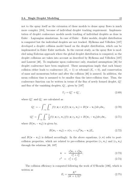
2.4. Single Droplet Modeling 43
not to the spray itself as the extension of these models to dense spray flows is much
more complex [184], because of individual droplet tracking requirement. Implementation
of droplet coalescence models needs tracking of individual droplets as done in
Euler – Lagrangian simulations. In case of Euler – Euler models, droplet distribution
is computed but the individual droplets are not tracked. Hylkema and Villedieu [187]
developed a droplet collision model based on the droplet distribution, which can be
implemented in Euler–Euler methods. In the current study, as the spray flow is modeled
using Eulerian approach where the global droplet distribution is computed, so the
droplet collisions are taken into account as described by Hylkema and Villedieu [187]
and Laurent [46]. To emphasize upon coalescence only, standard assumptions [46] for
droplet coalescence have been employed. These assumptions imply that each binary
collision either leads to coalescence (E c = 1) or rebound (E c = 0), and conservation
of mass and momentum before and after the collision [46] is assured. In addition, the
mean collision time is assumed to be smaller than the inter-collision time. Thus, the
coalescence function can be written in terms of the flux of newly formed droplet, Q + c
and flux of the vanishing droplets, Q − c , given by [187]
Γ f = Q + c + Q − c , (2.69)
where Q + c and Q − c are calculated as
Q − c
∫ ∞
= −
−∞
∫ ∞
0
f(t, x; r, v)f(t, x; r 1 , v 1 ) × B(|v − v 1 |)dr 1 dv 1 , (2.70)
Q + c =
∫ ∞ ∫ ∞
−∞
where B(|v 1 − v 2 |) is given by,
0
1
2 f(t, x; r 1, v 1 )f(t, x; r 2 , v 2 ) × B(|v 1 − v 2 |)dr 1 dv 1 , (2.71)
B(|v 1 − v 2 |) = π(r 1 + r 2 ) 2 |v 2 − v 1 |E c , (2.72)
and B(|v − v 1 |) is defined accordingly. In the above equations, (r, v) refer to postcollision
properties, which are related to pre-collision properties (r 1 , v 1 ) and (r 2 , v 2 )
through the relations [46, 187]
v = r3 1v 1 + r2v 3 2
, (2.73)
r1 3 + r2
3
r 3 = r1 3 + r2. 3 (2.74)
The collision efficiency is computed following the work of O’Rourke [186], which is
written as
E c =
K 2
(K + 1/2) 2 , (2.75)