Nuclear Spectroscopy

Gamma Energy (keV)
1400
1200
1000
800
600
400
200
X energy (keV)
X XXXX
linear fit
quadratic fit
X
X X X XXX
0
0 100 200 300 400 500 600
Channel Number
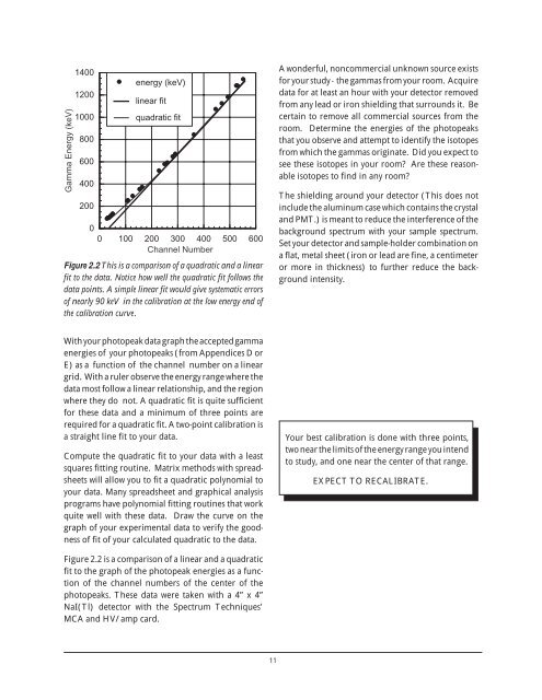
Figure 2.2 This is a comparison of a quadratic and a linear
fit to the data. Notice how well the quadratic fit follows the
data points. A simple linear fit would give systematic errors
of nearly 90 keV in the calibration at the low energy end of
the calibration curve.
A wonderful, noncommercial unknown source exists
for your study - the gammas from your room. Acquire
data for at least an hour with your detector removed
from any lead or iron shielding that surrounds it. Be
certain to remove all commercial sources from the
room. Determine the energies of the photopeaks
that you observe and attempt to identify the isotopes
from which the gammas originate. Did you expect to
see these isotopes in your room? Are these reasonable
isotopes to find in any room?
The shielding around your detector (This does not
include the aluminum case which contains the crystal
and PMT.) is meant to reduce the interference of the
background spectrum with your sample spectrum.
Set your detector and sample-holder combination on
a flat, metal sheet (iron or lead are fine, a centimeter
or more in thickness) to further reduce the background
intensity.
With your photopeak data graph the accepted gamma
energies of your photopeaks (from Appendices D or
E) as a function of the channel number on a linear
grid. With a ruler observe the energy range where the
data most follow a linear relationship, and the region
where they do not. A quadratic fit is quite sufficient
for these data and a minimum of three points are
required for a quadratic fit. A two-point calibration is
a straight line fit to your data.
Compute the quadratic fit to your data with a least
squares fitting routine. Matrix methods with spreadsheets
will allow you to fit a quadratic polynomial to
your data. Many spreadsheet and graphical analysis
programs have polynomial fitting routines that work
quite well with these data. Draw the curve on the
graph of your experimental data to verify the goodness
of fit of your calculated quadratic to the data.
Your best calibration is done with three points,
two near the limits of the energy range you intend
to study, and one near the center of that range.
EXPECT TO RECALIBRATE.
Figure 2.2 is a comparison of a linear and a quadratic
fit to the graph of the photopeak energies as a function
of the channel numbers of the center of the
photopeaks. These data were taken with a 4” x 4”
NaI(Tl) detector with the Spectrum Techniques’
MCA and HV/amp card.
11