Nuclear Spectroscopy

More documents

Recommendations

Info

SUPPLIES • NaI(Tl) detector with MCA • Radioactive sources: 22 Na, 54 Mn, 60 Co, 65 Zn, 88 Y, 133 Ba, 134 Cs, 137 Cs, 207 Bi SUGGESTED EXPERIMENTAL PROCEDURE 1. Start the MCA and check the calibration using the 137 Cs source. The observed photopeak should be centered near 661.6 keV. If it is not within 10 keV of the accepted value, you may need to recalibrate your system. 2. Place another source on the fourth shelf under the detector and acquire a spectrum with the full vertical scale at 1,000 counts. 3. Select a Region Of Interest (ROI) around your photopeak. Details for doing this are in Appendix A. Record the centroid of the photopeak and its FWHM. This is available to you by displaying the Peak Summary, or for the ROI where the cursor is located, by selecting the Display Region button to the right of the displayed spectrum. 4. Repeat step 3 for all the sources available to you. You may use all the data from Experiment #2 to avoid retaking spectra. DATA ANALYSIS From your data of photopeak energies and corresponding FWHM calculate the fractional resolution and graph its square as a function of the inverse of the corresponding photopeak energy. Use a linear least squares program to get the equation for the best straight line fit to your data. Graph this equation on the graph with your data. Is your fit to the data a good fit? Another way to test the theoretical explanations for the fractional resolution is to graph the natural logarithm of the fractional resolution as a function of the natural logarithm of the corresponding photopeak energy. Obtain the slope and intercept from a linear least squares fit to the data. 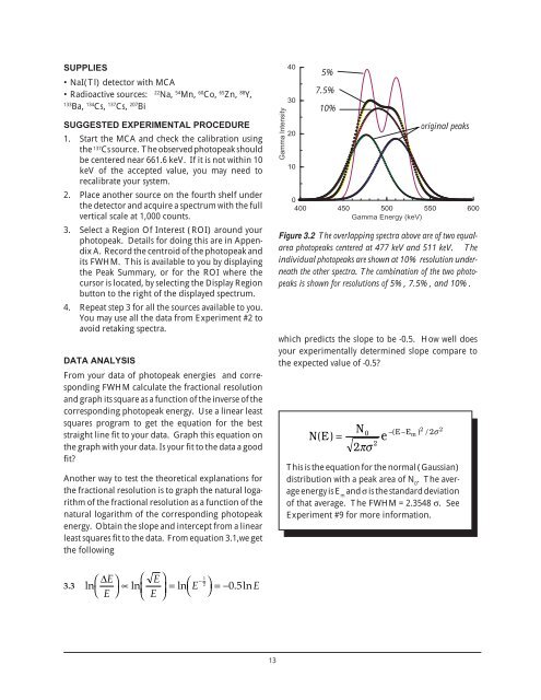From equation 3.1,we get the following Gamma Intensity 40 30 20 10 0XXXX 5% 7.5% 10% 400 450 500 550 600 Gamma Energy (keV) Figure 3.2 The overlapping spectra above are of two equalarea photopeaks centered at 477 keV and 511 keV. The individual photopeaks are shown at 10% resolution underneath the other spectra. The combination of the two photopeaks is shown for resolutions of 5%, 7.5%, and 10%. which predicts the slope to be -0.5. How well does your experimentally determined slope compare to the expected value of -0.5? NE ( ) = N 0 2πσ 2 2 −( e E − E m ) / 2σ 2 original peaks This is the equation for the normal (Gaussian) distribution with a peak area of N 0 . The average energy is E m and σ is the standard deviation of that average. The FWHM = 2.3548 σ. See Experiment #9 for more information. 3.3 ⎛ ∆E⎞ E ln ln ln E . lnE ⎝ E ⎠ ∝ ⎛ ⎝ ⎜ ⎞ E ⎟ ⎠ = ⎛ − 1 2 ⎞ ⎝ ⎠ =−05 13
E X P E R I M E N T 4 Compton Scattering INTRODUCTION There is more structure in your spectra than the photopeaks used in the last few experiments. Looking back at an earlier spectrum of 137 Cs, you will notice a small peak, or more precisely an edge, at about 477 keV. This is marked as the Compton Edge in Figure 4.1. Depending upon the geometrical arrangement of your detector and source, there is probably a photopeak at about 185 keV. There is only one gamma energy from 137 Cs, yet the observed spectrum has a photopeak at 661.6 keV, and these two Compton structures, an edge at 477 keV and a peak at 185 keV. How does this happen? It is due to Compton scattering by electrons. The Compton effect is a “collision” of the gamma photon with an atomic electron in which relativistic mass-energy and momentum are conserved. After the collision, the electron can have a kinetic energy that is a large fraction of the gamma’s original energy, E γ . The gamma loses this energy, becoming a lower frequency wave with energy, E γ ’ . The relation between the gamma’s energy before the collision compared to after the collision is 4.1 1 1 ( 1− cos θ) − = 2 Eγ ′ Eγ m e c Figure 4.2. Compton-scattering collision between an incoming photon, E γ , and a stationary electron. This results in a lower energy photon, E γ’ , scattered through angle θ, and the electron scattered through angle φ. where m e c 2 is the rest mass energy of the electron (511 keV) and θ is the angle through which the gamma is deflected. A depiction of the Compton scattering is shown in Figure 4.2. What is the origin of the Compton edge at 477 keV? A gamma enters the crystal of the detector and Compton scatters off an electron. The Compton-scattered gamma leaves the detector, so the amount of detected energy is the kinetic energy given to the electron. The maximum kinetic energy given to the electron, E max , results from a “head-on” collision with the gamma, scattering the gamma photon backwards (θ = 180 o ). From equation 4.1 this maximum electron energy is X rays Backscatter Photopeak Figure 4.1. Gamma spectrum from the decay of 137 Cs. Compton Edge 14
Page 1 and 2: Experimental γ Ray Spectroscopy an
Page 3 and 4: Published by Spectrum Techniques Al
Page 5 and 6: I N T R O D U C T I O N INTRODUCTIO
Page 7 and 8: Cardwell, and especially Robert Bra
Page 9 and 10: OBJECTIVE Calibrate the gamma-ray s
Page 11 and 12: E X P E R I M E N T 2 Gamma Spectra
Page 13: E X P E R I M E N T 3 Detector Ener
Page 17 and 18: DATA ANALYSIS, A CLASSICAL APPROACH
Page 19 and 20: Figure 5.3. Spectrum for the β −
Page 21 and 22: SUPPLIES •NaI(Tl) detector with M
Page 23 and 24: 14 12 X-Ray Energy (keV) 10 8 6 4 2
Page 25 and 26: E X P E R I M E N T 8 Multichannel
Page 27 and 28: E X P E R I M E N T 9 Counting Stat
Page 29 and 30: E X P E R I M E N T 10 Absolute Act
Page 31 and 32: gammas. This is true for 22 Na and
Page 33 and 34: E X P E R I M E N T 11 Potassium 40
Page 35 and 36: Exercise 11.2 Potassium in Fertiliz
Page 37 and 38: tern mantles, will have observably
Page 39 and 40: is needed. The activities of all is
Page 41 and 42: E X P E R I M E N T 13 Uranium 238
Page 43 and 44: 1 0.8 which is coincident with the
Page 45 and 46: of this type data, more is learned
Page 47 and 48: SUPPLIES •Some form of air pump t
Page 49 and 50: Exercise 14.4 Nuclear Fission Sever
Page 51 and 52: Table 14.1 Gamma-emitting Radioisot
Page 53 and 54: INSTALLATION ON A MACINTOSH MICROCO
Page 55 and 56: Regions of Interest. Region of inte
Page 57 and 58: Position the marker at the channel
Page 59 and 60: View Settings The VIEW SETTINGS men
Page 61 and 62: First acquire a spectrum of the sam
Page 63 and 64: Na I (Tl) D2 Electrons Anode θ θ
Page 65 and 66:
the multichannel analyzer’s typic
Page 67 and 68:
The solutions to these coupled diff
Page 69 and 70:
A P P E N D I X D Radioactive Decay
Page 71 and 72:
7/2+ 137 55 Cs 93.5% β 30.0 y - 90
Page 73 and 74:
A P P E N D I X E List of Commonly
Page 75 and 76:
Energy Element Half Life Associated
Page 77 and 78:
Atomic K α1 Energy K α2 Energy K-
Page 79 and 80:
C. Hohenemser and I. M. Asher,“A
Page 81:
General References. Nuclides and Is
show all

Nuclear Spectroscopy

You also want an ePaper? Increase the reach of your titles

Delete template?

Save as template?