

Multiattribute acceptance sampling plans - Library(ISI Kolkata ...
Multiattribute acceptance sampling plans - Library(ISI Kolkata ...
Multiattribute acceptance sampling plans - Library(ISI Kolkata ...

Create successful ePaper yourself
Turn your PDF publications into a flip-book with our unique Google optimized e-Paper software.
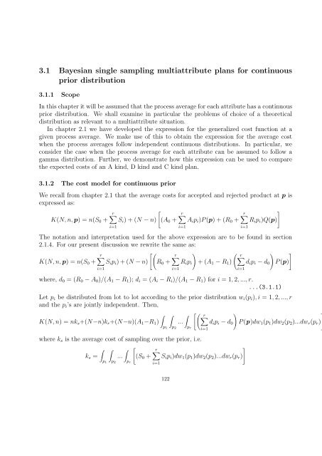
3.1 Bayesian single <strong>sampling</strong> multiattribute <strong>plans</strong> for continuous<br />
prior distribution<br />
3.1.1 Scope<br />
In this chapter it will be assumed that the process average for each attribute has a continuous<br />
prior distribution. We shall examine in particular the problems of choice of a theoretical<br />
distribution as relevant to a multiattribute situation.<br />
In chapter 2.1 we have developed the expression for the generalized cost function at a<br />
given process average. We make use of this to obtain the expression for the average cost<br />
when the process averages follow independent continuous distributions. In particular, we<br />
consider the case when the process average for each attribute can be assumed to follow a<br />
gamma distribution. Further, we demonstrate how this expression can be used to compare<br />
the expected costs of an A kind, D kind and C kind plan.<br />
3.1.2 The cost model for continuous prior<br />
We recall from chapter 2.1 that the average costs for accepted and rejected product at p is<br />
expressed as:<br />
[<br />
]<br />
r∑<br />
r∑<br />
r∑<br />
K(N, n, p) = n(S 0 + S i ) + (N − n) (A 0 + A i p i )P (p) + (R 0 + R i p i )Q(p)<br />
i=1<br />
The notation and interpretation used for the above expression are to be found in section<br />
2.1.4. For our present discussion we rewrite the same as:<br />
[(<br />
) (<br />
r∑<br />
r∑<br />
r∑<br />
) ]<br />
K(N, n, p) = n(S 0 + S i p i ) + (N − n) R 0 + R i p i + (A 1 − R 1 ) d i p i − d 0 P (p)<br />
i=1<br />
i=1<br />
where, d 0 = (R 0 − A 0 )/(A 1 − R 1 ); d i = (A i − R i )/(A 1 − R 1 ) for i = 1, 2, ..., r.<br />
...(3.1.1)<br />
i=1<br />
i=1<br />
Let p i be distributed from lot to lot according to the prior distribution w i (p i ), i = 1, 2, ..., r<br />
and the p i ’s are jointly independent. Then,<br />
∫ ∫ [( r∑<br />
) ]<br />
K(N, n) = nk s +(N−n)k r +(N−n)(A 1 −R 1 ) ... d i p i − d 0 P (p)dw 1 (p 1 )dw 2 (p 2 )...dw r (p r )<br />
∫p 1 p 2 p r i=1<br />
where k s is the average cost of <strong>sampling</strong> over the prior, i.e.<br />
∫ [<br />
]<br />
r∑<br />
k s = ... (S 0 + S i p i )dw 1 (p 1 )dw 2 (p 2 )...dw r (p r )<br />
∫p 1 p 2<br />
∫p r i=1<br />
i=1<br />
122


