Multiattribute acceptance sampling plans - Library(ISI Kolkata ...
Multiattribute acceptance sampling plans - Library(ISI Kolkata ...
Multiattribute acceptance sampling plans - Library(ISI Kolkata ...
You also want an ePaper? Increase the reach of your titles
YUMPU automatically turns print PDFs into web optimized ePapers that Google loves.
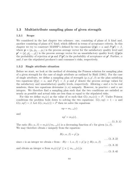
1.3 <strong>Multiattribute</strong> <strong>sampling</strong> <strong>plans</strong> of given strength<br />
1.3.1 Scope<br />
We considered in the last chapter two schemes: one, consisting of <strong>plans</strong> of A kind and,<br />
another consisting of <strong>plans</strong> of C kind, which differed in terms of <strong>acceptance</strong> criteria. In this<br />
chapter we try to construct MASSP’s defined by two equations Q(p) = α and P (p ′ ) = β,<br />
where p = (p 1 , p 2 , ..., p r ) is the process average vector for the satisfactory quality level and<br />
p ′ = (p ′ 1, p ′ 2, ..., p ′ r) is the process average vector for an unsatisfactory quality level; Q(p)is<br />
the probability of rejection at p and P (p ′ ) is the probability of <strong>acceptance</strong> at p ′ . Further, α<br />
and β are the stipulated producer’s and consumer’s risks, respectively.<br />
1.3.2 Single attribute situation<br />
Before we start, we look at the method of obtaining the Poisson solution for <strong>sampling</strong> plan<br />
of a given strength for the case of single attribute as outlined by Hald (1981). For the case<br />
of single attribute, we define a <strong>sampling</strong> plan of strength (p, α, p ′ , β) as the plan satisfying<br />
two equations Q(p) = α, and P (p ′ ) = β, p and p ′ denote the process average values for<br />
the satisfactory and unsatisfactory quality levels, respectively. Allowing c and n to be real<br />
numbers, these two equations determine (c, n) uniquely. However, in practice c and n are<br />
integers. We therefore find a <strong>sampling</strong> plan such that the two conditions are satisfied as<br />
nearly as possible and actual risks are less than or equal to the stipulated risks.<br />
For this we define m P (c) as the value of m such that G(c, m P (c)) = P . Under Poisson<br />
conditions the problem boils down to solving the two equations: G(c, np) = 1 − α and<br />
G(c, np ′ ) = β. Let G(c, m P (c)) = P then we solve the equations<br />
and<br />
np = m 1−α (c)<br />
np ′ = m β (c).<br />
...(1.3.1)<br />
The ratio R(c, α, β) = m β (c)/m 1−α (c) is a decreasing function of c for given (α, β).<br />
We may therefore obtain c uniquely from the equation:<br />
R(c, α, β) = p ′ /p<br />
since c is an integer we obtain c from : R(c − 1, α, β) > p ′ /p ≥ R(c, α, β)<br />
and obtain an integer n from m β (c)/p ′ ≤ n ≤ m 1−α (c)/p<br />
...(1.3.2)<br />
...(1.3.3)<br />
...(1.3.4)<br />
64


