B - St. Cloud State University

Ryan’s MFP-3D Procedural Operation ‘Manualette’ Version 10 (v080501; Igor 6.04A); 11.7
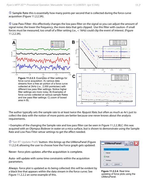
Sample Rate-this is essentially how many points per second that is collected during the force curve
acquisition (Figure 11.2.2.3A).
Low Pass Filter- this effectively changes the low pass filter on the signal so you can adjust the amount of
signal noise; the lower the frequency, the more data that gets clipped. Use this filter with caution- if small
forces must be measured, too small of a filter setting (i.e., < 1kHz) could clip the event of interest. (Figure
11.2.2.3A).
-1.35
A
-1.40
bl0012BW=500Hz
bl0014BW=1kHz
bl0020BW=20kHz
bl0027BW=50kHz
B
0.5
bl0038BW=200Hz; 10k Pt/s
bl0031BW=500Hz; 2k Pt/s
bl0036BW=1kHz; 5k Pt/s
bl0027BW=50kHz; 2k Pt/s
Force pN
-1.45
-1.50
Force pN
0.0
-0.5
-1.55
-1.0nN
-1.60
-1.65nN
7.24 7.23 7.22 7.21 7.20
µm
Figure 11.2.2.3: Examples of filter settings for
force curve acquisition: A) various data
streams from a free air portion of a force curve
collected at 2kHz (i.e., 2,000 points/sec) with
different low pass filter settings- Notice higher
filter settings are more noisy; B) Examples of
force curves collected at various sample Rates
and low pass filter settings: C) zoom of boxed
area in B).
C
Force pN
-300
-350
-400
-450
6.80 6.78 6.76 6.74 6.72 6.70
µm
bl0038BW=200Hz; 10k Pt/s
bl0031BW=500Hz; 2k Pt/s
bl0036BW=1kHz; 5k Pt/s
bl0027BW=50kHz; 2k Pt/s
-500pN
6.76 6.75 6.74 6.73
µm
The author typically sets the sample rate to at least twice the Nyquist Rate, but often as much as 4x’s just to
collect the data with the notion of more points are better because one never knows about the analysis
requirements.
• Examples of the changing the Sample rate and low pass filter can be seen in Figure 11.2.2.3B,C: this was
acquired with an Olympus Biolever in water on a mica surface, but is shown to demonstrate using the Sample
Rate and Low Pass Filter setvar settings to get the effect needed.
7 ‘Set RT Update Prefs’ button- this brings up the UiMenuPanel (Figure
11.2.2.4) allowing the user to choose how the Force graph gets updated:
Never- force plots updates after the acquisition is complete.
Auto- will update with some time constraints within the acquisition
parameters.
Always- force plot is updated as its being collected; this will be evident by
a black line that appears within the data stream in the force curve; See
Figure 11.2.2.2 an some example of this.
Figure 11.2.2.4: Real time
updating of force plots using the
UiMenuPanel.