A comparative study of models for predation and parasitism

48
animals when the prey densities were increased. My factor a(X) suggests that in
the case of parasitism, in which satiation might not be important, a deviation from
the observed would become greater as host density became higher.
Now, the handling-time factor h can be incorporated into my model by eliminating
t~ from eqs. (4c. 2) and (4e. 7), i.e.
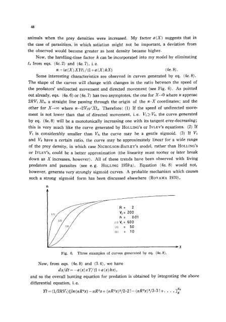
n = {a (X) XYt}/{1 + a (X) hX} (4e. 8).
Some interesting characteristics are observed in curves generated by eq. (4e. 8).
The shape of the curves will change with changes in the ratio between the speed of
the predators' undirected movement and directed movement (see Fig. 6). As pointed
out already, eqs. (4e. 6) or (4e. 7) has two asymptotes, the one for X-~0 where n approac
2RVI Xt,, a straight line passing through the origin of the n-X coordinates; and the
other for X~oo where n-~2V~v'Xt,. Therefore: (1) If the speed of undirected movement
is not lower than that of directed movement, i.e. V~ > V~, the curve generated
by eq. (4e. 8) will be a monotonically increasing one with its tangent ever-decreasing;
this is very much like the curve generated by HOLLING'S or IVLEV'S equations. (2) If
Va is considerably smaller than V2, the curve may be a gentle sigmoid. (3) If V1
and V~ have a certain ratio, the curve may be approximately linear for a wide range
of the prey density, in which case NICHOLSON-BAILEY'S model, rather than HOLLING'S
or IVLEV's, could be a better approximation (the Iinearity must sooner or later break
down as X increases, however). All of these trends have been observed with living
predators and parasites (see e.g. HOLLING 1959a). Equation (4e. 8) would not,
however, generate very strongly sigmoid curves. A probable mechanism which causes
such a strong sigmoid form has been discussed elsewhere (RoYAMA 1970).
R= 2
v2-- 200
h = 0.0'1
(~) V~ = 600
{2) = 50
{3) = 1 0
Fig. 6. Three examples of curves generated by eq. (4e. 8).
:~X
Now, from eqs. (4e. 8) and (3. 4), we have
dx/dt = -a (x) xY/ {1 +a (x) hx} ,
and so the overall hunting equation for predation is obtained by integrating the above
differential equation, i.e.
Yt = (1/2R V1) [ln (nR 2x) - nR 2x + (nR 2x) 2/2.21 - (nR ~x) 3/3.3 ! + ....
]xo