Multiscale Modeling of Theta ' Precipitation in Al-Cu Binary Alloys

2982 V. Vaithyanathan et al. / Acta Materialia 52 (2004) 2973–2987
the semi-coherent and coherent interfaces for the two
precipitate variants
0 ij ð1Þ ¼
11ð1Þ 0
¼ d
sc 0
;
0 22 ð1Þ 0 d c
0 ij ð2Þ ¼
11ð2Þ 0
¼ d
ð27Þ
c 0
;
0 22 ð2Þ 0 d sc
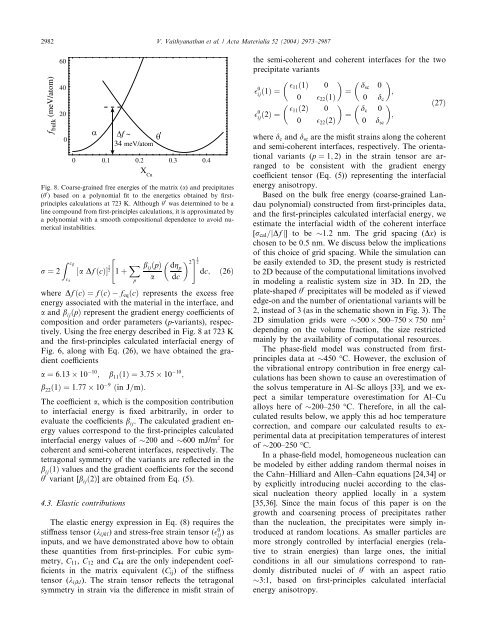
Fig. 8. Coarse-grained free energies of the matrix (a) and precipitates
(h 0 ) based on a polynomial fit to the energetics obtained by firstprinciples
calculations at 723 K. Although h 0 was determined to be a
line compound from first-principles calculations, it is approximated by
a polynomial with a smooth compositional dependence to avoid numerical
instabilities.
Z "
cb
r ¼ 2 ½a Df ðcÞŠ 1 2
1 þ X #1
b ij ðpÞ dg 2 2
p
dc; ð26Þ
c a
a dc
p
where Df ðcÞ ¼f ðcÞ f eq ðcÞ represents the excess free
energy associated with the material in the interface, and
a and b ij ðpÞ represent the gradient energy coefficients of
composition and order parameters (p-variants), respectively.
Using the free energy described in Fig. 8 at 723 K
and the first-principles calculated interfacial energy of
Fig. 6, along with Eq. (26), we have obtained the gradient
coefficients
a ¼ 6:13 10 10 ; b 11 ð1Þ ¼3:75 10 10 ;
b 22 ð1Þ ¼1:77 10 9 ðin J=mÞ:
The coefficient a, which is the composition contribution
to interfacial energy is fixed arbitrarily, in order to
evaluate the coefficients b ij . The calculated gradient energy
values correspond to the first-principles calculated
interfacial energy values of 200 and 600 mJ/m 2 for
coherent and semi-coherent interfaces, respectively. The
tetragonal symmetry of the variants are reflected in the
b ij ð1Þ values and the gradient coefficients for the second
h 0 variant [b ij ð2Þ] are obtained from Eq. (5).
4.3. Elastic contributions
The elastic energy expression in Eq. (8) requires the
stiffness tensor (k ijkl ) and stress-free strain tensor ( 0 ij )as
inputs, and we have demonstrated above how to obtain
these quantities from first-principles. For cubic symmetry,
C 11 , C 12 and C 44 are the only independent coefficients
in the matrix equivalent (C ij ) of the stiffness
tensor (k ijkl ). The strain tensor reflects the tetragonal
symmetry in strain via the difference in misfit strain of
where d c and d sc are the misfit strains along the coherent
and semi-coherent interfaces, respectively. The orientational
variants (p ¼ 1; 2) in the strain tensor are arranged
to be consistent with the gradient energy
coefficient tensor (Eq. (5)) representing the interfacial
energy anisotropy.
Based on the bulk free energy (coarse-grained Landau
polynomial) constructed from first-principles data,
and the first-principles calculated interfacial energy, we
estimate the interfacial width of the coherent interface
[r cal =jDf j] to be 1.2 nm. The grid spacing (Dx) is
chosen to be 0.5 nm. We discuss below the implications
of this choice of grid spacing. While the simulation can
be easily extended to 3D, the present study is restricted
to 2D because of the computational limitations involved
in modeling a realistic system size in 3D. In 2D, the
plate-shaped h 0 precipitates will be modeled as if viewed
edge-on and the number of orientational variants will be
2, instead of 3 (as in the schematic shown in Fig. 3). The
2D simulation grids were 500 500–750 750 nm 2
depending on the volume fraction, the size restricted
mainly by the availability of computational resources.
The phase-field model was constructed from firstprinciples
data at 450 °C. However, the exclusion of
the vibrational entropy contribution in free energy calculations
has been shown to cause an overestimation of
the solvus temperature in Al–Sc alloys [33], and we expect
a similar temperature overestimation for Al–Cu
alloys here of 200–250 °C. Therefore, in all the calculated
results below, we apply this ad hoc temperature
correction, and compare our calculated results to experimental
data at precipitation temperatures of interest
of 200–250 °C.
In a phase-field model, homogeneous nucleation can
be modeled by either adding random thermal noises in
the Cahn–Hilliard and Allen–Cahn equations [24,34] or
by explicitly introducing nuclei according to the classical
nucleation theory applied locally in a system
[35,36]. Since the main focus of this paper is on the
growth and coarsening process of precipitates rather
than the nucleation, the precipitates were simply introduced
at random locations. As smaller particles are
more strongly controlled by interfacial energies (relative
to strain energies) than large ones, the initial
conditions in all our simulations correspond to randomly
distributed nuclei of h 0 with an aspect ratio
3:1, based on first-principles calculated interfacial
energy anisotropy.