Multiscale Modeling of Theta ' Precipitation in Al-Cu Binary Alloys
Multiscale Modeling of Theta ' Precipitation in Al-Cu Binary Alloys
Multiscale Modeling of Theta ' Precipitation in Al-Cu Binary Alloys

Create successful ePaper yourself
Turn your PDF publications into a flip-book with our unique Google optimized e-Paper software.
2976 V. Vaithyanathan et al. / Acta Materialia 52 (2004) 2973–2987<br />
2.4. Phase-field model<br />
In the phase-field methodology, a precipitate microstructure<br />
is described by a set <strong>of</strong> cont<strong>in</strong>uum order parameter<br />
fields characteriz<strong>in</strong>g the difference <strong>in</strong> composition<br />
and structure between the precipitate and matrix [11]. In a<br />
two-dimensional representation <strong>of</strong> h 0 precipitates <strong>in</strong> a<br />
b<strong>in</strong>ary <strong>Al</strong>–<strong>Cu</strong> alloy, the precipitate microstructure is described<br />
by one composition field and two orientation-related<br />
long range order parameter fields.<br />
The chemical free energy <strong>of</strong> the microstructure, <strong>in</strong>clud<strong>in</strong>g<br />
the bulk and <strong>in</strong>terfacial energy, is then expressed<br />
as<br />
Z<br />
F bulk þ F <strong>in</strong>t ¼ f ðc; g 1 ; g 2 ; g 3 Þ þ a 2 ðrcÞ2<br />
V<br />
þ 1 X<br />
b<br />
2 ij ðpÞr i g p r j g p<br />
!dV ; ð4Þ<br />
p<br />
where a and b ij ðpÞ are gradient energy coefficients for<br />
composition and order parameters, respectively. b ij ðpÞ is<br />
reta<strong>in</strong>ed as a second rank tensor to <strong>in</strong>corporate the<br />
(tetragonal) anisotropy <strong>in</strong> <strong>in</strong>terfacial energy. The<br />
anisotropy <strong>in</strong> <strong>in</strong>terfacial energy <strong>of</strong> the precipitate is dependent<br />
on the orientational variant, g, <strong>of</strong> the precipitate<br />
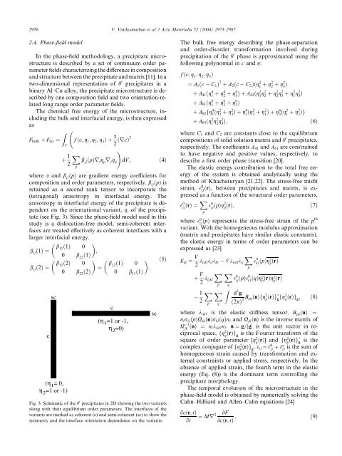
(see Fig. 3). S<strong>in</strong>ce the phase-field model used <strong>in</strong> this<br />
study is a dislocation-free model, semi-coherent <strong>in</strong>terfaces<br />
are treated effectively as coherent <strong>in</strong>terfaces with a<br />
larger <strong>in</strong>terfacial energy.<br />
<br />
b ij ð1Þ ¼ b <br />
11ð1Þ 0<br />
;<br />
0 b 22 ð1Þ<br />
<br />
b ij ð2Þ ¼ b <br />
11ð2Þ 0<br />
0 b 22 ð2Þ<br />
c<br />
sc<br />
(η 1 = 0,<br />
η 2 =1 or -1)<br />
<br />
¼ b <br />
22ð1Þ 0<br />
:<br />
0 b 11 ð1Þ<br />
c<br />
(η 1 =1 or -1,<br />
η 2 =0)<br />
ð5Þ<br />
Fig. 3. Schematic <strong>of</strong> the h 0 precipitates <strong>in</strong> 2D show<strong>in</strong>g the two variants<br />
along with their equilibrium order parameters. The <strong>in</strong>terfaces <strong>of</strong> the<br />
variants are marked as coherent (c) and semi-coherent (sc) to show the<br />
symmetry and the <strong>in</strong>terface orientation dependence on the variants.<br />
sc<br />
The bulk free energy describ<strong>in</strong>g the phase-separation<br />
and order-disorder transformation <strong>in</strong>volved dur<strong>in</strong>g<br />
precipitation <strong>of</strong> the h 0 phase is approximated us<strong>in</strong>g the<br />
follow<strong>in</strong>g polynomial <strong>in</strong> c and g:<br />
f ðc; g 1 ; g 2 ; g 3 Þ<br />
¼ A 1 ðc C 1 Þ 2 þ A 2 ðc C 2 Þðg 2 1 þ g2 2 þ g2 3 Þ<br />
þ A 41 ðg 4 1 þ g4 2 þ g4 3 ÞþA 42ðg 2 1 g2 2 þ g2 2 g2 3 þ g2 1 g2 3 Þ<br />
þ A 61 ðg 6 1 þ g6 2 þ g6 3 Þ<br />
þ A 62 fg 4 1 ðg2 2 þ g2 3 Þþg4 2 ðg2 3 þ g2 1 Þþg4 3 ðg2 1 þ g2 2 Þg<br />
þ A 63 ðg 2 1 g2 2 g2 3 Þ;<br />
ð6Þ<br />
where C 1 and C 2 are constants close to the equilibrium<br />
compositions <strong>of</strong> solid solution matrix and h 0 precipitates,<br />
respectively. The coefficients A 41 and A 61 are constra<strong>in</strong>ed<br />
to have negative and positive values, respectively, to<br />
describe a first order phase transition [20].<br />
The elastic energy contribution to the total free energy<br />
<strong>of</strong> the system is obta<strong>in</strong>ed analytically us<strong>in</strong>g the<br />
method <strong>of</strong> Khachaturyan [21,22]. The stress-free misfit<br />
stra<strong>in</strong>, 0 ijðrÞ, between precipitates and matrix, is expressed<br />
as a function <strong>of</strong> the structural order parameters,<br />
0 ij ðrÞ ¼X 0 ij ðpÞg2 p ðrÞ;<br />
ð7Þ<br />
p<br />
where 0 ijðpÞ represents the stress-free stra<strong>in</strong> <strong>of</strong> the pth<br />
variant. With the homogeneous modulus approximation<br />
(matrix and precipitates have similar elastic constants),<br />
the elastic energy <strong>in</strong> terms <strong>of</strong> order parameters can be<br />
expressed as [23]<br />
E el ¼ V 2 k X<br />
ijkl ij kl V k ijkl ij 0 kl ðpÞg2 p ðrÞ<br />
þ V 2 k X X<br />
ijkl 0 ij ðpÞ0 kl ðqÞg2 p ðrÞg2 q ðrÞ<br />
1 X<br />
2<br />
p<br />
p<br />
q<br />
X<br />
Z<br />
q<br />
p<br />
d 3 g<br />
ð2pÞ 3 B pqðnÞfg 2 p ðrÞg g fg2 q ðrÞg g ;<br />
ð8Þ<br />
where k ijkl is the elastic stiffness tensor. B pq ðnÞ ¼<br />
n i r ij ðpÞX jk ðnÞr kl ðqÞn l and X jk ðnÞ is the <strong>in</strong>verse matrix <strong>of</strong><br />
X 1<br />
jk ðnÞ ¼ n ik ijkl n l . n ¼ g=jgj is the unit vector <strong>in</strong> reciprocal<br />
space, fg 2 q ðrÞg g<br />
is the Fourier transform <strong>of</strong> the<br />
square <strong>of</strong> order parameter [g 2 q ðrÞ] and fg2 p ðrÞg g<br />
is the<br />
complex conjugate <strong>of</strong> fg 2 p ðrÞg g . ij ¼ 0 ij þ a ij<br />
is the sum <strong>of</strong><br />
homogeneous stra<strong>in</strong> caused by transformation and external<br />
constra<strong>in</strong>ts or applied stress, respectively. In the<br />
absence <strong>of</strong> applied stra<strong>in</strong>, the fourth term <strong>in</strong> the elastic<br />
energy (Eq. (8)) is the dom<strong>in</strong>ant term controll<strong>in</strong>g the<br />
precipitate morphology.<br />
The temporal evolution <strong>of</strong> the microstructure <strong>in</strong> the<br />
phase-field model is obta<strong>in</strong>ed by numerically solv<strong>in</strong>g the<br />
Cahn–Hilliard and <strong>Al</strong>len–Cahn equations [24]<br />
ocðr; tÞ<br />
ot<br />
¼ Mr 2 dF<br />
dcðr; tÞ ;<br />
ð9Þ