110 / 210 Fiber Optic Oxygen Monitor - Instech Laboratories, Inc.

Fiber Optic Oxygen Monitor 

Models 110 and 210 

Operating Manual 

110-210 manual v6.doc 

Printed 4.8.2003 

Most current version is available online at 

http://www.instechlabs.com/manuals.html 

Instech Laboratories, Inc. 

5209 Militia Hill Road 

Plymouth Meeting PA 19462 

USA 

TL 800-443-4227 or 610-941-0132 

FX 610-941-0134 

www.instechlabs.com 

Featuring technology from: 

Some of the text and images in this 

manual are courtesy of Ocean Optics, Inc. 

Software installation precautions-Order is very important 

See page 11 

With no USB connected—Install software but do not run 

Attach USB 

Run software. 

1

Table of Contents 

Software installation precautions-Order is very important .................................................................................................. 1 

System Overview............................................................................................................................................................................3 

Summary of Setup Procedure .................................................................................................................................................... 4 

System Assembly............................................................................................................................................................................5 

Monitor Assembly ....................................................................................................................................................................... 5 

125 Series Probe Assembly ....................................................................................................................................................... 5 

Instech Series 600 Chambers......................................................................................................................................................6 

Titanium Micro Chamber Assembly........................................................................................................................................7 

Introduction.................................................................................................................................................................................. 7 

Water Jacket Plumbing............................................................................................................................................................... 8 

Stirring Motor Installation.......................................................................................................................................................... 8 

Titanium Chamber Insertion and Removal............................................................................................................................. 8 

Installing the Probe...................................................................................................................................................................... 8 

Chamber Plugs............................................................................................................................................................................. 9 

Using the Titanium Chamber with O-ring fitted plugs with central fill hole.................................................................. 10 

Software Overview.......................................................................................................................................................................11 

Software Installation...................................................................................................................................................................12 

Software Operation .....................................................................................................................................................................14 

Display Functions...................................................................................................................................................................... 15 

File Menu Functions................................................................................................................................................................. 18 

Configure Menu Functions...................................................................................................................................................... 18 

Graph & Chart Menu Functions ............................................................................................................................................. 22 

Spectrometer Menu Functions ................................................................................................................................................ 23 

Probe Calibration.........................................................................................................................................................................24 

Physical Calibration Setup....................................................................................................................................................... 24 

Calibration Procedure ............................................................................................................................................................... 24 

INTAKE Utility Software..........................................................................................................................................................26 

Other Probes .................................................................................................................................................................................27 

Appendix 1: Theory of Operation ...........................................................................................................................................28 

Appendix 2: Hardware Descriptions ......................................................................................................................................31 

S2000-series Pin-outs and Jumpers ........................................................................................................................................ 31 

USB2000-series Pin-outs ......................................................................................................................................................... 33 

R-LS-450 Rack-mount Blue LED Pulsed Light Source..................................................................................................... 33 

SAD500 Specifications ............................................................................................................................................................ 35 

125/FO Probe Specifications................................................................................................................................................... 35 

Appendix 3: Chemical Effects on FOXY Probes ...............................................................................................................36 

2

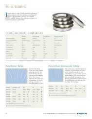
System Overview 

The Model 110 is a single channel monitor 

containing 1 Serial A/D card, 1 light source card, 1 

spectrometer card, 1 bifurcated fiber optic cable and a 

power supply. The Model 210 adds an extra light 

source, spectrometer and fiber optic cable. 

These systems incorporate the latest in fiber optic 

probe technology to detect and record the 

concentration of oxygen, either in gaseous form or 

dissolved in liquids. Oxygen is sensed by the 

quenching of fluorescence of an indicator dye trapped 

in a matrix at the tip of the probe. Since this is an 

equilibrium measurement, there will be no "motion 

artifact" as is seen with polarographic electrodes. The 

fluorophore is excited by a pulsed blue LED light 

source and the resulting fluorescence is detected 

using a miniature spectrometer. The OOISensors 

software controls the spectrometer, light sources, 

display and data logging. 

Probes can be provided in several configurations. The 

125/FO version has the same external dimensions as 

our 125 series polarographic electrodes and is 

physically interchangeable, except for some flow 

cells. The tip of the probe is coated with an opaque 

layer of black silicone. The coating permits use in 

ambient light. No electrolytes or replaceable 

membranes are required. Other probes as small as 

500 micron OD are available. 

How it Works 

Light from the blue LED travels from the "out" port, 

down the fiber to the probe where it excites the 

fluorescent dye. Some blue light is returned along 

with the fluorescence and travels back up the fiber to 

the "in" port where it enters a miniature spectrometer. 

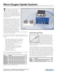
The diagram below shows a typical spectral trace and 

some explanation of the parameters that you will be 

using in setting up the monitor. The dye fluoresces 

most brightly when no oxygen is present and 

decreases with increasing oxygen concentration. 

Oxygen as a triplet molecule is able to quench 

efficiently the fluorescence and phosphorescence of 

certain luminophores. This effect (first described by 

Kautsky in 1939) is called "dynamic fluorescence 

quenching." Collision of an oxygen molecule with a 

fluorophore in its excited state leads to a nonradiative 

transfer of energy. The degree of 

fluorescence quenching relates to the frequency of 

collisions, and therefore to the concentration, 

pressure and temperature of the oxygen-containing 

media. 

The graphs below illustrate how the raw intensity 

signal is converted within the software to a linear 

output by use of the Stern-Volmer linearizaton. 

Appendix 1 covers the equations governing the 

linearizaton and temperature corrections. 

Max 4096 

~600 nm 

3

3500 

3000 

Raw Fluoroscence vs [O] 

250 

[O] vs Io/I 

Stern Volmer Linearization 

2500 

200 

Intensity 

2000 

1500 

1000 

500 

0 

0 50 100 150 200 250 

Oxygen Concentration [O] 

[O] 

150 

100 

50 

0 

1 1.2 1.4 1.6 1.8 2 

Io/I 

Summary of Setup 

Procedure 

• Setup up Monitor with power supply, serial 

cable, and bifurcated fibers and attach probes. 

For USB A/D converter version, do not attach 

USB cable to computer yet. 

• Install software (first time) 

• Attach USB cable. 

• Turn on Oxygen Monitor unit. 

• Configure hardware (first time). 

• Enter spectrometer wavelength calibration 

coefficients for each channel (first time). 

• Prepare calibration setup for one temperature and 

2 oxygen concentrations. 

• Do zero oxygen first and establish acquisition 

parameters for each probe. 

• Calibrate at ambient oxygen level for each probe. 

• Ready to run. 

4

System Assembly 

Monitor Assembly 

125 Series Probe Assembly 

For the SAD500 version the monitor requires that the 

DC power adapter be plugged into the rear as well as 

the RS-232 cable. Use the DIN to 9-pin adapter cable 

to attach the oxygen monitor to an available COM 

port on your PC. 

For USB version, just attach USB cable to computer 

after software has been installed. 

Attach the bifurcated ends of the fiber optic cable to 

the "out" and "in" SMA optical connectors on the 

front panel of the monitor. Use the tubular wrench to 

secure the fittings. The single end will attach to the 

probe via the ¾” sleeve coupler. If possible, keep the 

fiber optic cable positions the same once calibrated to 

avoid small errors due to cable differences. If using a 

dual system, keep the probes associated with a given 

channel once calibrations have been performed. 

Positions are labeled A, B..., on the Monitor front 

panel to facilitate this. Switches on the rear are 

disabled. 

The 125/FO is a silica-core, 1000-µm stainless steel 

fiber optic probe with a 1/8" outer diameter and an O- 

ring seal and 2.5" in length It is designed for use with 

a 600-µm bifurcated optical fiber assembly. 

Caution! 

♦ Avoid using ketones (acetone and alcohols 

included) with the 125/FO. 

♦ Handle with care. Dropping the probe may cause 

permanent damage. 

♦ Gently remove the plastic cover from the SMA 

connector before use. Cleaning 

♦ Sterilize the 125/FO by gamma radiation or 

ETO. If you sterilize the probe, you must 

recalibrate. 

♦ You can use detergents to clean the probe. Using 

detergents to clean the probe does not necessitate 

calibration. 

♦ Avoid cleaning the 125/FO with ketones 

(acetone and alcohols included) or organic 

solvents. 

Assembly 

The tip of the probe is covered with a thin layer of 

black silicone. Care must be exercised to prevent 

puncturing or peeling of this layer. To prepare the 

125/FO for use in Instech compatible systems, slide 

the threaded sleeve over the electrode first. Load O- 

ring onto the installing tool and place the tool over 

the end of the probe. Push the O-ring off and into the 

groove. The probe can now be installed into the 

chamber and the sleeve tightened to form a seal and 

hold it in place. 

5

Installing the o-ring on the 125/FO probe. 

Removing the o-ring from 125/FO probe. WARNING: 

cut it rather than trying to push it off over the tip. It is 

better to sacrifice the O-ring rather than to damage 

the tip coating. 

Instech Series 600 

Chambers 

Setting Up the Batch Cell Chamber 

The batch cell mode uses the chamber cup with a 

magnetic stirring motor mounted behind it. The 

chamber cup is sealed with the window valve that is 

held in place by a thin layer of silicone grease. 

1. Plug in the speed controller. Plug the AC 

adapter into the DC IN jack of the speed 

controller first, then plug the AC adapter into a 

wall outlet. 

2. Plug the motor into MOTOR OUT jack of the 

speed controller. The motor should run when 

the speed controller is turned on. 

3. Temporarily insert the chamber cup into the 

chamber block. Push in the red leak protection 

divider from the rear of the chamber block using 

a pencil until it hits the chamber cup. The 

opening should face away from the chamber cup. 

4. Insert the motor/magnet assembly into the 

chamber block until it hits the red spacer, then 

pull it back about 1 mm. 

5. Gently tighten the set screw to hold the motor 

using the provided allen wrench. 

Silicone 

grease 

6. Insert the chamber cup into the front of the 

chamber block. 

7. Place the stir bar into the chamber cup. It 

should couple to the magnet and rotate freely 

against the back of the cup when the speed 

controller is turned on. 

8. Apply a small amount of silicone grease to the 

flat front surface of the chamber cup. Avoid the 

small fill and overflow port holes. 

9. Press the window against the cup and rotate it to 

distribute the grease uniformly across the face. 

10. Pull off the window valve and clean off excess grease 

from the inside of cup using a toothpick. Check the 

port holes as well. Do not clean the layer of grease 

from the face of the cup – this will form the seal for 

the window. 

Uniformly 

distributed 

6

11. Clean off all grease from the window valve. An 

acetone dampened tissue works well. 

12. Press the window valve back on to the chamber cup 

and rotate to distribute the grease across the face. 

13. Install the appropriate fill port plug into the top of the 

chamber. If you plan to use a plastic-tipped 

micropipette to add fluid to the chamber during 

your experiment, use the single-piece pipette 

plug. If you plan to use a microliter syringe, use 

the two-piece syringe plug. 

from the chamber block and that the setscrew does not 

protrude into the hole. 

2. Attach inlet and outlet tubes of your experiment to the 

flow cell. The system is designed for 1/16” ID tubing, 

such as Tygon.The flow cell is now ready for the 

probe. 

Pipette Fill 

Port Plug 

Hamilton Syringe 

Fill Port Plug 

The chamber is now ready for the electrode. When 

inserted, the electrode will hold the cup firmly in 

place. 

Setting up the Flow Cell 

Chamber 

Flow cell chamber assembly 

The various pieces of equipment designed for the batch cell 

mode (i.e., speed controller, motor, chamber cup, window 

valve, and red spacer) are not needed and should be set 

aside. 

Most in-line experiments involve measuring the difference 

in oxygen level at two points in a sy stem, and thus will 

require that you set up two flow cells. 

To set up the flow cell chamber: 

1. Insert the flow cell into the chamber block from the 

front. Be sure that batch cell parts have been removed 

Titanium Micro 

Chamber 

Assembly 

Introduction 

This chamber is constructed of non-reactive titanium 

with volumes of 250 microliters to 1 ml. It is top 

loading for easy sample loading and clean out. A 

beveled, transparent, sample-sealing plug serves also 

as a valve by closing off the angled fill port when 

rotated. The angle on the plug allows air to be easily 

purged. An alternative acrylic plug with a central fill 

hole may also be provided. Miniature stirring system 

and a nickel/Teflon coated aluminum block are 

standard. Stirring is not required to achieve a stable 

reading with this type of probe but faster thermal 

equilibrium will be achieved and any particulates will 

be kept in suspension. 

7

Water Jacket Plumbing 

1. Use 5/16” ID Tygon tubing on the two outboard 

fittings. 

2. Secure in place using clamps or cable ties. 

3. If the center coupling should require changing, 

remove the stirring motor from one block, 

remove the block mounting screws and attach 

short length of tubing between the inner block 

fittings. Again secure tubing. DO NOT 

ATTEMPT THIS WITH THE PROBE IN PLACE. 

Stirring Motor Installation 

1. Loosen the motor holding setscrew (lower front 

center of block) until it does not protrude into the 

bore. 

2. Back off the chamber holding setscrew and 

temporarily place the titanium chamber into the 

top of the aluminum block. 

3. From the bottom, insert the motor/magnet 

assembly and push it until it contacts the bottom 

of the titanium chamber. 

4. Pull the motor back about 1 mm and gently 

tighten the motor holding setscrew. Excessive 

force will damage the motor. 

Titanium Chamber Insertion 

and Removal 

1. Drop chamber into opening at the top of the 

block with the fiber entry hole in the rear and 

roughly aligned with the threaded hole that will 

accept the fiber sealing screw. 

2. Use the fiber sealing screw (without the fiber and 

seal) to set the alignment by screwing it into the 

block until seated. Some rotation of the chamber 

may be necessary. 

3. The length of 22 ga.. stainless steel hypodermic 

tubing should be inserted prior to installing the 

probe in check the alignment once the seal is in 

place. Place the seal over the end of the tubing. 

4. When the seal screw is seated, tighten the front 

chamber holding setscrew. This will assure that 

the tip of the fiber will not be damaged when 

inserted subsequently. The seal will remain in 

the hole once the tubing is removed. 

Installing the Probe 

Note: At all times take care not to damage the fiber 

probe. 

1. Attach the probe to the unmounted L-bracket by 

screwing it into the ¾” hollow sleeve coupler. 

Fiber will be on the side nearest the L-bracket 

tightening screw. Do not attach the bifurcated 

bundle yet. Before tightening the probe, rotate it 

until the black angled face is upward to minimize 

light leakage. 

2. Place the bracket with probe installed on the 

groove in the back supporting rail. 

3. Loosen the seal tightening screw so that the 

probe will pass through the seal without friction. 

8

4. Loosen the bracket thumbscrew and place the 

bracket in the track. 

5. Very carefully slide the probe through the hole in 

the seal tightening screw and advance it until the 

tip just protrudes into the chamber. Do not allow 

the tip to touch the far side of the well, it could 

jam and crack the tip. 

6. The final position of the probe tip should have 

just the angled portion of the tip exposed with 

the bevel facing upward. As the seal is tightened, 

it may advance into the chamber. Tighten seal 

and then reposition as necessary until the seal no 

longer can be moved. 

Chamber Plugs 

Depending upon the chamber size, different style 

plugs may be use, either beveled tip style or O-ring 

style with single vertical fill hole. 

The beveled type can be rotated to seal off the side 

fill hole. 

For large volume chambers, e.g. 1000 microliters, the 

central hole can be plugged to reduce oxygen leakage 

although little reoxygenation actually occurs. 

Larger chambers have no side fill hole. 

Setting the Optional Beveled Plug Depth 

1. Slide a fine tip micro pipette tip into the fill hole 

until it touches the far side of the chamber well. 

2. Drop the beveled transparent plug into the well 

with the bevel matching the angle of the pipette 

tip. 

3. Place the collar over the plug and tighten the 

holding screw facing forward. This will be the 

position indicator as well. 

4. This process will position the depth of the plug 

so that air will clear properly when the chamber 

is initially filled 

7. Repeat for the second chamber and then attach 

the single end of each bifurcated fiber bundle. 

Using the Titanium Micro 

Chamber with Beveled Plug 

1. Fill the chamber with buffer solution that has 

been equilibrated at your operating temperature 

with the oxygen tension to be used in the 

experiment. Use slightly more than the specified 

9

volume of the chamber. A small overflow will 

occur. 

2. If working at ambient pO 2, you may allow some 

time to allow thermal and oxygen equilibration 

to occur before sealing off the sample. 

3. Add cells or organelles and slide in the central 

transparent core plug. Orient the top collar so 

that the air rises to the top of the bevel and exits 

through the fill port. 

4. The setscrew should be facing you when the plug 

has been correctly installed. 

5. Turn off stirring, if on. 

6. Slowly continue to slide the plug down while 

watching from above to ensure that all air is 

expelled from the chamber. 

7. When no air bubbles are visible, rotate the top 

collar until the setscrew faces toward the rear 

which will seal the chamber. 

8. Additions can made though the fill port in the 

right front of the chamber. First return the 

plug/valve to the forward position to allow entry. 

9. This should be done with a loosely fitting needle 

or pipette so that the overflow will flow by the 

needle. No separate vent port is needed. Inject 

near the bottom and the overflow will flow out 

from the top part of the chamber and into the 

circular trough. Turning the stirrer off during this 

procedure is recommended to reduce mixing. 

Using the Titanium 

Chamber with O-ring fitted 

plugs with central fill hole. 

This type does not depend on the use of the side fill 

hole and may not even exist with larger chambers. 

1. Fill chamber with plug out to slightly more than 

the stated chamber volume. 

2. Gently push plug into chamber. Air should be 

expelled and a small amount of solution will be 

expelled insuring that no bubbles remain. 

3. Continue as in step 9 above. 

10

Software Overview 

This software is designed to operate Instech 

Laboratories Model 110 or 210 Fiber Optic Oxygen 

Monitoring systems. These systems incorporate 

Ocean Optics' spectrometers, light sources and A/D 

boards. It is a native 32 bit application for Windows 

95, 98, NT and 2000. USB unit requires Windows 98, 

2000 or NT This version includes an optional second 

order Oxygen calibration to the linear regression 

(Stern-Volmer). Temperature calibration data is valid 

for gaseous measurements but not for dissolved 

oxygen. See Appendix 1 for procedures when 

measuring gaseous oxygen. 

The operating screen or “front panel” displayed on 

the PC monitor, is a virtual instrument with graphs, 

charts, controls and indicators. Depending on 

selection, it is possible to view the full wavelength 

spectrum, intensity or concentration time chart, 

current concentration values. This information can be 

viewed simultaneously for up to eight channels, 

although only Master and Slave1 are used in the 

Model 210 and Master only in the Model 110. 

Users have to do a single temperature Multipoint 

calibration - Linear/Polynomial, without temperature 

compensation for dissolved oxygen measurements. 

System settings are saved upon exiting the system. 

Once all settings have been established, exit and 

reenter the OOISensors program. They will then 

become the defaults next time the program is started. 

Calibration routines will save to their files during the 

operation of the program. 

Nominal Setup Parameters-Adjust as needed 

Spectrometer type* 

A/D converter type* 

USB Serial Number* 

Channel Active 

Scan dark for every 

measurement 

Sensor 

Chart 

Nm 

Bandwidth 25 

Pressure compensation 

Temperature measurement 

Enable Reference correction 

Wavelength coefficients* 

Subtract dark box 

S2000/PC2000… 

ADC1000USB 

Select detected 

Check for each 

check 

Foxy 

sensor 

Peak wavelength 

None 

None 

unchecked 

Fill from sheet 

check 

Integ. time 64-512 

Average 2 

Boxcar smooth 10 

Scan 

Calculate sensor values with 

scan 

Calibrate 

Temp compensation 

Calibration type 

* Required first time 

Continuous 

Pull downchecked 

Oxygen, single 

temperature 

no 

Multi Point 

11

Load the software using the Password provided. 

Software 

Installation 

The following files are included on the CD 

provided: 

110-210 Manual v6.pdf Operating manual 

Websetup.exe 

Sets up and installs software 

Intake Demo 

Used as oxygen partial pressure 

or content calculator-old DOS 

program but front end is useful 

SAD500 Serial Port Interface Version 

You have this version if the unit shipped with a round 

DIN to DB9 RS-232 cable. 

The SAD500 Serial Port Interface is a 

microprocessor-controlled A/D converter for serial 

port connection or stand-alone operation. The 

SAD500 can be used to interface to desktop or 

portable PCs, PLCs and other devices that support the 

RS-232 communication protocol. The following are 

directions for setting up your SAD500. Because A/D 

converter installation goes hand-in-hand with 

software installation, you will find directions for 

installing OOISensors Software in this section as 

well. 

Interface the SAD500 to your PC 

Interfacing the SAD500 to a desktop or portable PC 

is simple. 

1. If your 110 or 210 came equipped with a 

SAD500 mounted onto your spectrometer, 

simply connect the 6-pin DIN end of the serial 

cable to the SAD500 and the DB9 end to your 

PC. 

2. For either configuration, note the serial port 

number (also called COM Port) on the PC to 

which you are interfacing. (Older PCs may not 

have numbered ports.) 

3. Plug the +12VDC wall transformer into an outlet 

and connect it to the power jack on the rear of 

the monitor unit. 

ADC1000-USB Interface Version 

Overview 

Do not attach USB cable until software has been 

loaded. 

Attach USB cable to computer and monitor. 

Windows should recognize USB connection. 

Only now should you run the software. 

This is the newer of the two versions and will ship 

with units after Jan. 1, 2002. This version requires a 

USB port on your computer and is shipped with the 

appropriate USB cable. 

1. Plug 12VDC power supply to rear of monitor 

unit. You may leave this turned off at this time. 

2. Plug the flat end of the USB cable into the 

computer and leave the monitor end of the cable 

unconnected for now. 

Install OOISensors 

Before installing OOISensors, make sure that no 

other applications are running. Also, make sure you 

have the OOISensors password, which can be found 

on the CD cover. During installation, you will have to 

enter this password. 

1. Execute Websetup.exe . At the "Welcome" 

dialog box, click Next> 

2. At the "Destination Location" dialog box, accept 

the default or choose Browse to pick a directory. 

Click Next> 

3. At the "Backup Replaced Files" dialog box, 

select either Yes or No. We recommend 

choosing Yes. If you select Yes, you can choose 

Browse to pick a destination directory. Click 

Next>. 

4. Select a Program Manager Group. Click Next>. 

At the "Start Installation" dialog box, click 

Next>. 

5. At the "Installation Complete" dialog box, 

choose Finish>. Restart your computer after 

installation is complete. 

6. You may wish to create a shortcut and drag it to 

the desktop. 

Configuring for SAD500 

After restarting your computer, turn the monitor unit 

on and then start OOISensors. 

The first time you run OOISensors after installation, 

you will need to initialize some parameters. 

12

Configure Hardware Dialog Box 

your information in

Configuring ADC1000-USB 

Note: ORDER IS IMPORTANT. After restarting 

your computer, first turn the monitor unit on and 

attach USB cable to the rear of the 110 or 210 

monitor. Initiate OOISensors. 

The first time you run OOISensors after installation, 

select the Configure Hardware dialog box. 

1. Select Configure | Hardware from the menu. 

The parameters in this dialog box are usually set 

only once -- when OOISensors is first installed 

and the software first runs. 

2. Under Spectrometer Type 

S2000,PC2000,HR2000 

3. Under A/D Converter Type, choose ADC1000- 

USB. 

4. Under USB Serial Number, select the 

spectrometer serial number, this should match 

the calibration sheet number. 

5. Select Configure|Spectrometer, activate the 

channel/s you will be using and check that the 

spectrometer coefficients appear as on the 

calibration sheet provided. If they do not match, 

enter each value and exit the program to save 

these values to non-volatile ram on the 

ADC1000. 

Software Operation 

OOISensors Software is our next generation of 

operating software for our FOXY Fiber Optic Oxygen 

Sensing systems. OOISensors is a 32-bit, advanced 

acquisition and display program that provides a realtime 

interface to a variety of signal-processing 

functions for Windows 95/98/2000/NT users. With 

OOISensors, users have the ability to obtain oxygen 

partial pressure and concentration values, control all 

system parameters, collect data from up to 8 

spectrometer channels simultaneously and display the 

results in a single spectral window, perform time 

acquisition experiments and display and correct for 

temperature fluctuations in the sample. 

The most important change from the previous oxygen 

sensing software, the 16-bit OOIFOXY, is the ability 

to use the Second Order Polynomial algorithm in the 

calibration procedure. This algorithm often provides 

more accurate data than the linear Stern-Volmer 

algorithm. Also, with OOISensors, you can now 

monitor temperature. The software corrects the data 

for any fluctuations in temperature. Another 

improvement over OOIFOXY is that OOISensors can 

display up to 8 spectrometer channels in one spectral 

window, and yet each spectrometer channel can have 

its own data acquisition parameters. 

What's more, a time chart displays the data from all 

active channels at a specific wavelength over time. 

During a timed data acquisition procedure, you can 

enter text for an event into the log file. Enabling the 

time chart and the data logging function are as easy 

as clicking on switches next to the graph. 

14

Display Functions 

Several functions are accessed not through the menu 

but through buttons and taskbars directly on the 

display window, on the top and to the right of the 

spectral graph and time chart areas. From the display 

window, you can choose a mode to acquire data, take 

scans of your sample, store a dark spectrum, 

configure the cursor, configure the graph, enter data 

acquisition parameters and analyze data. Scan Single 

and Continuous 

When in Single mode, the Scan function acts as a 

snapshot. After selecting the Single mode, click the 

Scan switch to ON to take a scan of the sample. The 

switch stays in the ON position until the scan has 

been completed (the time set in the Integration Time 

box). The switch then moves to the OFF position. 

When in Cont. (continuous) mode, 

the recommended setting, the Scan 

function continuously takes as many 

scans of the sample as needed. After 

each integration cycle, another scan 

will immediately begin. Click the switch to OFF to 

discontinue acquiring data. 

Store Dark 

This function stores the current 

spectrum as the dark spectrum 

for all active channels 

It is not necessary to use this function as long as the 

Subtract Dark box is checked Configure | 

Spectrometer from the menu, click on the Sensors 

tab and select Scan dark for every measurement. 

When this function is enabled, while the LS-450 

automatically turns off, and a dark scan is stored, 

each time you take a sample scan. 

Subtract Dark 

Selecting this box subtracts the current dark spectrum 

from the spectra being displayed. This command is 

useful if you are trying to eliminate from the spectra 

fixed pattern noise caused by a very long integration 

time. This function is only for display purposes. It 

should be checked along with Scan dark for every 

measurement. 

15

Data Acquisition Parameters 

When altering parameters, turn scan to OFF to speed 

up program response to your actions. 

Functions at the top of the display window such as 

choosing the integration time, averaging and boxcar 

smoothing values provide you with immediate access 

to important data acquisition settings. 

Channel [CH] 

To set the data acquisition parameters (such as 

integration time, averaging and boxcar 

smoothing) for a specific spectrometer channel, 

first select the spectrometer channel from the CH 

pull down menu. This pull down menu is not for 

selecting the spectrometer channels that are 

active in the display graph; it's only for setting 

data acquisition values for each channel. (To 

activate your spectrometer channels and have 

them displayed, select Configure | 

Spectrometer from the menu and click on the 

Sensors tab. Enable each spectrometer in your 

system.) 

Integration Time 

Enter a value to set the integration time in 

milliseconds for the chosen spectrometer 

channel. The integration time of the spectrometer 

is analogous to the shutter speed of a camera. 

The higher the value specified for the integration 

time, the longer the detector "looks" at the 

incoming photons. If your signal intensity is too 

low, increase this value. If the signal intensity is 

too high, decrease the value. Adjust the 

integration time until the fluorescence peak 

(~600 nm) is about 1500-2000 counts in air or 

saturated water. The fluorescence peak should 

not exceed 3500 counts when oxygen is absent. 

The intensity of the LED peak (~475 nm) does 

not affect your measurements. You only need to 

adjust the integration time if the fluorescence 

peak is saturating the detector. 

Average 

Enter a value to implement a sample averaging 

function that averages the specified number of 

spectra for the chosen spectrometer channel. The 

higher the value entered the better the signal-tonoise 

ratio (S:N). The S:N improves by the 

square root of the number of scans averaged. 

Boxcar Smooth 

Enter a value to implement a boxcar smoothing 

technique that averages across spectral data for 

the spectrometer channel chosen. This method 

averages a group of adjacent detector elements. 

A value of 5, for example, averages each data 

point with 5 points (or bins) to its left and 5 

points to its right. The greater this value, the 

smoother the data and the higher the signal-tonoise 

ratio. However, if the value entered is too 

high, a loss in spectral resolution results. The 

S:N improves by the square root of the number 

of pixels averaged. When using the oxygen 

sensors, we recommend setting the boxcar 

smoothing value to no more than 25 pixels. 

Cursor Functions 

In this bar, you can label the cursor, monitor its X 

and Y values and move the cursor. To the right of the 

X and Y values of the cursor is a cursor selection 

button that allows you to choose a cursor style and a 

point style. 

+ Sign 

When the + is selected, the pointer becomes a 

crosshair symbol, enabling you to drag the cursor 

around the graph. 

Magnify Symbols 

There are several magnify functions from which 

to choose. The function chosen remains in use 

until another magnify icon or the crosshair 

symbol is selected. Clockwise, beginning with 

the top left symbol, the magnify icons perform 

the following functions: 

1. magnifies a specific area by clicking and 

dragging a box around the area 

16

2. zooms in on the horizontal scale, but the 

vertical scale remains the same 

3. zooms in on the vertical scale, but the 

horizontal scale remains the same 

4. zooms in approximately one point vertical 

and horizontal, click once or press 

continuously 

5. zooms out approximately one point vertical 

and horizontal, click once or press 

continuously 

6. reverts to the last zoom function 

Cursor Diamonds 

To move the cursor left or right in small 

increments in the graph area, click on the left and 

right cursor diamonds. 

Cursor Label 

The first box in the configure cursor taskbar 

allows you to label the cursor. 

X and Y Values 

The cursor taskbar displays the X value and Y 

value of the cursor point. 

Cursor Properties 

To the right of the X and Y values of the 

cursor is a cursor selection button that 

allows you to utilize many cursor features such 

as choosing a cursor style, selecting a point style 

and finding a color for the cursor trace. 

Data Values 

Spectral Graph 

The data displayed to the 

right of the graphs and chart 

areas provides you with the 

oxygen values for each 

spectrometer channel and 

probe combination. If you 

are monitoring and 

correcting for temperature, 

these values appear in this 

area as well. 

The spectral graph area of the display window 

provides you with real-time spectral scans of your 

sample. You can change the vertical and/or 

horizontal scales of the graph by simply clicking on 

an X and Y endpoint and manually typing in a value. 

The graph will then resize itself. 

Temperature Chart 

To display the temperature chart, select 

Graph&Chart | View Temperature Chart from 

the menu. The Temperature Chart will then take the 

place of the Spectral Graph. To save the 

Temperature Chart, select File | Save Time Chart 

from the menu. You will receive two Save prompts, 

one for the Time Chart and one for the Temperature 

Chart. By selecting Graph&Chart | View 

Temperature Chart again (deselecting the 

function), the Spectral Graph will return. 

You can also save Temperature Chart data without 

displaying the chart. By selecting Configure | 

Spectrometer from the menu, clicking on the Sensors 

tab, and enabling the Chart function under 

Temperature Measurement, temperature data is 

collected, whether or not the Temperature Chart is 

displayed. Then you can use the save function. 

Time Chart 

The time chart displays the data from all active 

channels at a specific wavelength over time. To view 

the Time Chart, select Configure | Spectrometer 

from the menu and click on the Display tab. Make 

sure that Spectral Graph & Time Chart is selected 

next to Graph and Chart Display Mode . To 

configure a timed data acquisition procedure, select 

Configure | Spectrometer from the menu and click 

on the Timing tab. (For details on configuring a timed 

acquisition procedure, see page 53.) 

Time Chart and Log On/Off Switches 

Once you have configured a 

timed data acquisition 

procedure, you can start and 

stop the acquisition by clicking 

on the Time Chart switch. 

(To set the parameters for a timed data acquisition 

procedure, select Configure | Spectrometer from the 

menu, click on the Timing tab and enter your 

settings.) Turn on and off saving this data to a log file 

by clicking on the Log switch. (To set parameters for 

saving timed acquisition data, select Configure | 

Spectrometer from the menu, click on the Log tab, 

select how frequently you want to save data and 

choose the file name for the log.) Only the last 

10,000 scans of a timed data acquisition can be saved 

in the log file. 

17

File Menu Functions 

Save Spectrum 

Select File | Save Spectrum from the menu to save 

the current spectrum as a tab-delimited ASCII file. 

You can then open these files as overlays in the 

spectral graph or import them into other software 

programs, such as Microsoft Excel. 

Configure Menu Functions 

Hardware 

Save Time Chart 

Select File | Save Time Chart from the menu to save 

the current time chart as a tab-delimited ASCII file. 

You can then open these files as a static chart or 

import them into other software programs, such as 

Microsoft Excel. 

Open Spectrum 

Select File | Open Spectrum from the menu to open 

a dialog box that allows you to open a previously 

saved spectrum and to open it as an overlay (a static 

spectrum) while still acquiring live data. 

Open Time Chart 

Select File | Open Time Chart from the menu to 

open a dialog box that allows you to choose a 

previously saved time chart and open it as a static 

chart. 

Page Setup 

Select File | Page Setup to select printing 

parameters. 

Print Spectrum and Time Chart 

Select File | Print Spectrum from the menu to print 

the current display in the Spectral Graph, or select 

File | Print Time Chart from the menu to print the 

time chart. 

Exit 

Select File | Exit from the menu to quit OOISensors. 

A message box appears asking you if you are sure 

you want to exit the software. 

The Configure Hardware dialog box sets the hardware 

parameters for the spectrometer. The parameters in 

this dialog box are usually set only once -- when 

OOISensors is first installed. The first time you run 

OOISensors after installation, you need to select 

settings in the Configure Hardware dialog box. Select 

Configure | Hardware from the menu. First, select a 

Spectrometer Type (the S2000-FL, SF2000 and 

USB2000 are S2000-series spectrometers). Next, 

select an A/D Converter Type. Select the A/D 

converter you are using to interface your spectrometer 

to your computer. Your choices are the 

ADC500/PC1000, ADC1000/PC2000, DAQ700, 

SAD500, Serial USB2000 or USB2000. 

Depending on the Spectrometer Type and the A/D 

Converter Type you chose, other choices must be 

made: 

♦ For SAD500 users: 

-- Enter your computer’s Serial Port (or 

COM Port) number to which the device is 

connected. 

-- Select the Baud Rate or speed at which the 

device will operate. 

-- Enter a SAD500 Pixel Resolution, which 

specifies that every nth pixel of the 

spectrometer is transmitted from the 

SAD500 to the PC. Enter resolution values 

from 1 to 500. Your resolution value 

depends on your experiment. By sacrificing 

18

pixel resolution, you gain speed. The 

transfer of one complete spectra requires 

~0.4 seconds when communicating at 

115,200 baud rate. If you need your 

information in

♦ Analysis Wavelength Box. Enter the 

analysis wavelength. The analysis 

wavelength should be very close to 600 nm. 

(When the excited ruthenium complex at the 

tip of the oxygen probe fluoresces, it 

typically emits energy at ~600 nm.) In the 

Bandwidth [box] pixels area, select the 

number of pixels around the analysis 

wavelength to average. 

♦ Data Display for Sensor Measurement. 

Choose the data display format and 

precision of the data. Under Format select 

Decimal or Scientific. Under Precision, 

select a value to specify the precision of the 

oxygen data displayed and saved in files. 

The maximum is 5. 

♦ Wavelength Calibration Coefficients 

♦ Do not forget to enter these the first time 

using the system. 

Check the Wavelength Calibration Data Sheet 

that came with your system to make sure the 

values on the Data Sheet and in this dialog box 

are the same. If not, enter the coefficients 

otherwise spectral data may be skewed. 

♦ Pressure Compensation CH. If you have 

your own external pressure measuring 

system, you can use this feature to monitor 

and correct for pressure fluctuations in your 

sample. You can either use a pressure 

transducer separately from the system or 

interface it to your sensor system. If you 

interface a pressure transducer to your 

sensor system, you must have an available 

spectrometer channel that is not connected 

to an oxygen sensor. Use the pull down 

menu to select how you want to monitor 

pressure. See Spectrometer DB-25 

connector details for attaching the analog 

signal to an unused A/D input channel. 

♦ Temperature Measurement. If you want to 

monitor and correct for temperature 

fluctuations in your sample, select a method 

from the pull down menu. 

-- Select None if you are not monitoring 

temperature. For now, this is the 

recommended setting. 

-- Select Manual if you are monitoring 

temperature, but you do not want 

OOISensors Software to read and 

display the temperature values. The 

Manual selection means that you must 

manually type temperature values in the 

display window. Enable the 

Compensate function if you want the 

software to correct for temperature 

fluctuations only if you calculated the 

temperature coefficients. Enabling the 

Chart function allows you to view a 

chart of the temperature values. 

-- Select Omega D5xx1 RS232 if you are 

monitoring temperature and if you want 

the software to automatically read and 

display the temperature values. Ocean 

Optics offers the Omega Thermistor and 

the Omega Thermocouple for 

monitoring temperature. The thermistor 

and thermocouple should already be 

connected to your PC via an RS-232 

module. Next to Serial Port, select the 

COM Port number on your PC to which 

the thermistor or thermocouple is 

connected. Because the RS-232 module 

can support up to four thermistors or 

thermocouples, it has these four ports 

labeled. Next to D5xx1 CH, select the 

port to which the thermistor or 

thermocouple connects to the RS-232 

module. (If you only have one 

thermistor or thermocouple, select 0.) 

Enable the Compensate function if you 

want the software to correct for 

temperature fluctuations. Enabling the 

Chart function allows you to view a 

chart of the temperature values. 

♦ Enable reference correction. Disable this 

function. 

♦ Level alarm. Enable this feature to set 

alarm properties. A green indicator appears 

in the display window if this feature is 

activated. If the values fall below the alarm 

parameters, the green indicator turns red. If 

the values rise above the alarm parameters, 

the green indicator turns yellow. 

20

Timing Tab 

-- To synchronize data acquisition with 

external events, choose External 

Software Trigger. In this leveltriggered 

mode, the spectrometer is 

"free running," just as it is in the normal 

mode. With each trigger, the data 

collected up to the trigger event is 

transferred to the software. (See 

Appendix D for details.) 

♦ Once you have configured a timed data 

acquisition procedure, you can start and stop 

the acquisition by clicking on the Time 

Chart switch on the main display window. 

Display Tab 

To configure a timed data acquisition procedure, 

select Configure | Spectrometer from the menu 

and select the Timing tab. In this dialog box, 

you can set the parameters for a timed data 

acquisition procedure. 

♦ Preset Duration. Enable this box and enter 

values to set the length for the entire timed 

acquisition process. Be sure to enter hours 

(HH), minutes (MM) and seconds (SS). 

♦ Preset Sampling Interval. This is 

frequently used to reduce the number of data 

points saved to disk by inserting a delay 

between samples. Enable the Preset 

Sampling Interval box and enter a value to 

set the frequency of the data collected in a 

timed acquisition process. Be sure to select 

hours (HH), minutes (MM) and seconds 

(SS). 

♦ Flash Delay. (Normally not selected) Enter 

a value to set the delay, in milliseconds, 

between external strobe signals of the LS- 

450 Blue LED light source. You can only 

use this feature if you have an ADC1000 

A/D converter. 

♦ External Trigger Mode. (Not normally 

used).You have two methods of acquiring 

data. Choose a triggering mode from the pull 

down menu: 

-- In the normal mode (called No 

External Trigger), the spectrometer is 

continuously scanning, acquiring, and 

transferring data to your computer, 

according to parameters set in the 

software. In this mode, however, there 

is no way to synchronize the acquisition 

of data with an external event. 

To configure your display window, select 

Configure | Spectrometer from the menu and 

click on the Display tab. In this dialog box, 

select the graphs and charts to appear in the 

display window. 

♦ Graph and Chart Display Mode. Choose 

the information that appears in the display 

window. If you choose Spectral Graph 

Only, a spectral graph appears in the display 

window. If you choose Spectral Graph & 

Time Chart, the spectral graph appears in 

the top of the display window and the time 

chart appears in the bottom. (To view a 

temperature chart, select Graph&Chart | 

View Temperature Chart from the main 

menu. The temperature chart then replaces 

the spectral graph.) 

♦ Temperature Units. Select either Celsius 

or Fahrenheit as the temperature units. (The 

application works in Kelvin, and converts to 

Celsius or Fahrenheit.) 

♦ Color for overlays. Select colors for static 

spectra that open when selecting File | Open 

Spectrum from the menu. These static 

21

Log Tab 

spectra are called overlays and you may 

wish to distinguish overlays from real-time 

spectra by changing the colors of their 

traces. 

Graph & Chart Menu 

Functions 

Clear Spectrum Graph 

Select Graph&Chart | Clear Spectrum Overlays 

from the menu to remove static spectra from the 

graph. 

Clear Time Chart 

Select Graph&Chart | Clear Time Chart from 

the menu to clear the time chart traces. A message 

box then appears, asking if you are sure you want 

to clear the time chart. 

Enable Grid 

To configure the data logging feature for a timed data 

acquisition procedure, select Configure | 

Spectrometer from the menu and select the Log tab. 

♦ Store to disk every x acquisitions. Enter a 

value to set how many scans are stored in RAM 

before they are saved permanently into a file. 

The smaller this number, the more frequently 

data is saved permanently to a file. The larger 

this number, the less frequently data is saved 

permanently to a file, but entering a large 

number enhances the performance of the process. 

♦ Filename and Path. Name the log file for the 

timed data acquisition process. Click on the file 

folder icon to navigate to a designated folder. 

♦ Insert Event in Log File. If you want to enter 

text into the log file, you can select 

Spectrometer | Insert Event in Log File from 

the menu. A dialog box then appears allowing 

you to enter text. In the log file, this text appears 

next to the data that was acquired at the time you 

entered the text. 

♦ To turn the logging function on for the time 

chart, you must select the Log On/Off 

Switch on the main display window. 

Select Graph&Chart | Enable Grid from the menu 

to generate a grid in the spectral graph. If you also 

have the time chart displayed, this function will 

create a grid in the time chart as well. De-selecting 

Enable Grid from the menu makes the grid 

disappear. 

Autoscale Horizontal (Spectral Graph) 

Select Graph&Chart | Autoscale Horizontal 

(Spectral Graph) from the menu to automatically 

adjust the horizontal scale of a current graph so the 

entire horizontal spectrum fills the display area. 

Autoscale Vertical (Spectral Graph) 

Select Graph&Chart | Autoscale Vertical 

(Spectral Graph) from the menu to automatically 

adjust the vertical scale of a current graph so the 

entire vertical spectrum fills the display area. 

Autoscale Vertical (Time Chart) 

Select Graph&Chart | Autoscale Vertical (Time 

Chart) from the menu to automatically adjust the 

vertical scale of a current time chart so the entire 

vertical chart fills the display area. 

View Temperature Chart 

Select Graph&Chart | View Temperature Chart 

from the menu to view temperature data. The 

temperature chart replaces the spectral chart. To view 

the spectral graph again, select Graph&Chart | 

View Temperature Chart from the menu and the 

spectral graph replaces the temperature chart. 

22

Spectrometer Menu 

Functions 

Scan-usually Continuous 

Select Spectrometer | Scan from the menu to take a 

scan of your sample. When in Single mode, (seldom 

used) the Scan function acts as a snapshot. The button 

depresses and Stop replaces Scan. The button will stay 

depressed until the scan has been completed (the time 

set in the Integration Time box). 

When in Continuous mode, the Scan button 

continuously takes as many scans of the sample as 

needed. After each integration cycle, another scan 

immediately begins. The button depresses and Stop 

replaces Scan. Select Spectrometer | Scan from the 

menu or click on the Stop button to halt the scanning 

process and discontinue acquiring data. 

Insert Event in Log File 

During a timed data acquisition procedure, you can 

enter text into the log file by selecting Spectrometer 

| Insert Event in Log File. A dialog box then 

appears allowing you to enter text. In the log file, this 

text appears next to the data that was acquired at the 

time you entered the text. Both the Time Chart and 

Log switches in the display window should be turned 

to the On position to use this feature. 

Enable Strobe Not normally used 

If you have configured the spectrometer to control 

the LS-450 selecting this function in the software 

allows you to enable or disable the triggering of the 

LS-450 Blue LED light source. The value entered in 

Flash Delay of the Timing tab in the Configure 

Spectrometer dialog box sets the delay, in 

milliseconds, between strobe signals of the LS-450 

Blue LED light source. 

Calculate Sensor Values with Scan 

When you first start OOISensors, the values 

displayed in the Data Values boxes to the right of 

the Spectral Graph will appear illogical. These 

values will continue to appear this way until you 

have calibrated your system. If you don't want to see 

these illogical values displayed, deselect 

Spectrometer | Calculate Sensor Values with 

Scan. 

Once you have calibrated your system, this function 

should always be enabled (or have a check mark in 

front of it) if you want the oxygen values displayed. 

23

Probe Calibration 

Physical Calibration Setup 

Assemble a system that will maintain constant 

temperature of the medium and probe and a means of 

presenting known oxygen concentration to the probe. 

The easiest concentrations will be atmospheric 

oxygen levels (20.9%) and zero. Zero oxygen is best 

attained by adding sodium dithionite to the solution. 

This will chemically remove the oxygen. Bubbling 

with nitrogen or an inert gas is more difficult and 

fraught with pitfalls. Decide on the units of oxygen 

concentration you will be using. 

Included with the unit is equipment to facilitate the 

calibration procedure for dissolved oxygen levels if 

the OR125 series probes are being used. A black 

holder attached to a long ¼” handle has two holes for 

probes and one small hole for a thermocouple 

temperature monitoring device (user supplied). 

Calibration Procedure 

This procedure does not include temperature 

compensation as this not yet possible with dissolved 

oxygen measurements. 

1. Set data acquisition parameters for your 

calibration procedure, such as integration time, 

averaging and boxcar smoothing. 

2. Set the integration time for the entire calibration 

procedure when the probe is measuring the 

standard with zero concentration. The 

fluorescence peak (~600 nm) will be at its 

maximum at zero concentration. Adjust the 

integration time so that the fluorescence peak 

does not exceed 3500 counts. If your signal 

intensity is too low, increase the integration time. 

If the signal intensity is too high, decrease the 

integration time. Set the integration time to 

powers of 2 (2, 4, 8, 16, 32, 64, 128, 256, 512, 

etc.) to ensure a constant number of LED pulses 

during the integration time. The intensity of the 

LED peak [~475 nm] will not affect your 

measurements providing that compensation has 

24

not been enabled. It will affect readings if the 

LED peak becomes saturated and compensation 

is enabled. 

3. Select Calibrate | Oxygen, Single Temperature 

from the menu. 

4. Enter the serial number of the probe in the S/N 

box. Today's date should enter automatically in 

the Date box. The file name and path appears 

under Calibration File Path once you select 

File | Save Calibration Chart and save the 

chart. At the 

5. This area is for typing in a label; it does not 

affect data in any way. 

6. Next to Calibration Type , select Multi Point 

from the pull down menu. 

7. Under Channel, select the spectrometer channel 

to which the sensor you are calibrating is 

connected. 

8. Under Curve Fitting, select the kind of 

algorithm you want to use to calibrate your 

sensor system: Linear (Stern-Volmer) or 

Second Order Polynomial. Calibration curves are 

generated from your standards and the 

algorithms to calculate concentration values for 

unknown samples. The Second Order 

Polynomial algorithm provides a better curve fit 

and therefore more accurate data during oxygen 

measurements, especially if you are working in a 

broad oxygen concentration range. 

♦ If you choose Linear (Stern-Volmer), you 

must have at least two standards of known 

oxygen concentration. The first standard 

must have 0% oxygen concentration and the 

last standard must have a concentration in 

the high end of the concentration range in 

which you will be working. 

♦ If you choose Second Order Polynomial, 

you must have at least three standards of 

known oxygen concentration. The first 

standard must have 0% oxygen 

concentration and the last standard must 

have a concentration in the high end of the 

concentration range in which you will be 

working. Since achieving 3 known dissolved 

oxygen levels is usually difficult, this mode 

is not recommended. 

9. In the Calibration Table, in the Standard # 

column, enter 1 for your first standard of known 

oxygen concentration. The first standard should 

have 0% oxygen concentration, such as can be 

found in a nitrogen flow or in a solution of 

sodium hydrosulfite or sodium dithionite. 

10. Under the Concentration column, enter 0. 

11. Leave your FOXY probe in the standard for at 

least 5 minutes to guarantee equilibrium. 

Checking the continuous box will allow 

watching of Intensity values to ensure that they 

are stable. 

Calibration Data 

Once you have calibrated your sensor system, the 

calibration data is stored in two files. It is stored in 

the OOISensors.cfg file, which is the application 

configuration file. The calibration data is called from 

this binary file each time you use your sensor system 

and software. 

Calibration data is also stored in an ASCII file (or text 

file) so that you use read the data and even import it 

into other application programs such as Microsoft Word 

and Excel. This ASCII file is called chXFoxy.cal, 

where "X" stands for the spectrometer channel ("0" for 

master spectrometer, "1" for spectrometer channel 1, 

"2" for spectrometer channel 2 and so on). The 

chXFoxy.cal file is not used by the OOISensors 

application; it is strictly for analyzing calibration data. 

(If you have temperature data in this file, temperature 

will be displayed as Kelvin.) 

If you ordered the Factory Calibration, you are 

provided with an additional file that includes data for 

the Calibration Table in the Multiple Temperature 

Calibration dialog box. The name of the file 

corresponds to the serial number of the probe. Unless 

otherwise specified, these coefficients are applicable 

to gaseous measurements only. 

25

INTAKE Utility Software 

Installing INTAKE DEMO 

• Copy the files provided into a separate directory. 

No special setup is required. 

• Create a shortcut to demo.exe for desktop for 

ease of access. 

Using INTAKE DEMO 

This DOS program is provided as a tool to help 

calculate oxygen concentrations or partial pressures 

at different temperatures for the calibration process 

data entry. It was part of discontinued Instech 

Laboratories acquisition system but is helpful in 

performing calculations quickly. Disregard all but the 

“modify parameters” feature. Use the arrow keys to 

move around the screen. Use Gas -> Units to set units 

of measure. Enter temperature values to calculate 

concentration. Volume can be set to 1000 ml to read 

in micromolar. 

26

Other Probes 

Probes 

There are seven available oxygen probes. The distal 

tip of each probe is polished and coated with the 

oxygen-sensing material. The proximal end of each 

probe has an SMA 905 fitting for coupling to the 

optical cables. 

Overcoats 

The following silicone overcoats exclude ambient 

light, improve chemical resistance and eliminate 

refractive index effects. A silicone overcoat is 

required for applications involving liquids or gas-toliquid 

activity. 

Ocean Optics PN 

FOXY-OR125G 

FOXY-R 

FOXY-AL300 

FOXY-PI600 

FOXY-24G 

FOXY-OR125 

FOXY-T1000 

Description 

1000-µm core diameter stainless steel 

fiber optic probe, 1/8" outer diameter, 

O-ring groove at tip, 2.5" in length, 

designed to couple to a 600-µm 

bifurcated fiber and splice bushing 

(direct replacement for 1/8" diameter 

oxygen electrodes) This is the 

standard probe (125/FO) supplied with 

the Instech Laboratories Model 110 

and 210. 


optical fiber, 1/16" outer diameter 

stainless steel tube beveled at 45°, 

approximately 6" in length, designed to 

couple to a 600 µm bifurcated fiber 

and splice bushing 

300-µm aluminum jacketed fiber optic 

probe, 1 m in length, designed to 



600-µm polyimide coated fiber optic 

probe, 2 m in length, designed to 


and splice bushing These are available 

in customs lengths as well. 

300-µm aluminum jacketed fiber optic 

probe with 24-gauge needle tip for 

penetrating vial septa, designed to 

couple to a 200-µm bifurcated fiber 



fiber optic probe, 1/8" outer diameter, 

2.5" in length, designed to couple to a 

600-µm bifurcated fiber and splice 

bushing (direct replacement for 1/8" 

diameter oxygen electrodes) 


fiber optic probe with screw-on light 

shield, 1/4" outer diameter, 

approximately 7" in length, designed to 

couple to a 600-µm bifurcated fiber 


Ocean Optics PN 

FOXY-AF 

FOXY-AF-MG 

Description 

RTV healthcare-grade silicone 

overcoat for FOXY probes 

RTV high-strength medical implantgrade 

silicone overcoat for FOXY 

probes (provides a thicker and 

stronger coating than the FOXY-AF) 

Additional probes may be ordered directly from 

Instech Laboratories. 

27

Appendix 1: Theory of Operation 

Linear (Stern-Volmer) Algorithm 

The Stern-Volmer algorithm requires at least two 

standards of known oxygen concentration. The first 

standard must have 0% oxygen concentration and the 

last standard must have a concentration in the high 

end of the concentration range in which you will be 

working. The fluorescence intensity can be expressed 

in terms of the Stern-Volmer equation where the 

fluorescence is related quantitatively to the partial 

pressure of oxygen: 

I 0 

I 

= 1 + k p O2 

I 0 is the intensity of fluorescence at zero pressure 

of oxygen, 

I is the intensity of fluorescence at a pressure p 

of oxygen, 

k is the Stern-Volmer constant 

For a given media, and at a constant total pressure 

and temperature, the partial pressure of oxygen is 

proportional to oxygen mole fraction. 

The Stern-Volmer constant (k) is primarily dependent 

on the chemical composition of the ruthenium 

complex. Our probes have shown excellent stability 

over time, and this value should be largely 

independent of the other parts of the measurement 

system. However, the Stern-Volmer constant (k) does 

vary among probes, and it is temperature dependent. 

All measurements should be made at the same 

temperature as the calibration experiments or 

temperature monitoring devices should be used. 

If you decide to compensate for temperature, the 

relationship between the Stern-Volmer values and 

temperature is defined as: 

I 0 = a 0 + b 0 * T + c 0 * T 2 

k = a + b * T + c * T 2 

The intensity of fluorescence at zero pressure of 

oxygen (I 0 ) depends on details of the optical setup: 

the power of the LED, the optical fibers, loss of light 

at the probe due to fiber coupling, and backscattering 

from the sample. It is important to measure the 

intensity of fluorescence at zero pressure of oxygen 

(I 0 ) for each experimental setup. 

It is evident from the equation that the sensor will be 

most sensitive to low levels of oxygen. Deviations 

from the Stern-Volmer relationship occur primarily at 

higher oxygen concentration levels. Using the Second 

Order Polynomial algorithm when calibrating 

corrects these deviations. 

Second Order Polynomial Algorithm 

The Second Order Polynomial algorithm requires at 

least three standards of known oxygen concentration. 

The first standard must have 0% oxygen 

concentration and the last standard must have a 

concentration in the high end of the concentration 

range in which you will be working. 

The Second Order Polynomial algorithm is 

considered to provide more accurate because it 

requires at least three known concentration standards 

while the Linear (Stern-Volmer) algorithm requires a 

minimum of two known concentration standards. The 

Second Order Polynomial algorithm is defined as: 

I 0 

I 

= 1 + K 1 * [O] + K 2 * [O] 2 

I 0 is the fluorescence intensity at zero 

concentration 

I is the intensity of fluorescence at a pressure p 

of oxygen, 

K 1 is the first coefficient 

K 2 is the second coefficient 

If you decide to compensate for temperature, the 

relationship between the Second Order Polynomial 

algorithm and temperature is defined as: 

I 0 = a 0 + b 0 * T + c 0 * T 2 

K 1 = a 1 + b 1 * T + c 1 * T 2 

K 2 = a 2 + b 2 * T + c 2 * T 2 

Henry’s Law 

It is possible to calibrate the FOXY system in gas and 

then use the FOXY system in liquid or vice versa. In 

theory, your FOXY system detects the partial 

pressure of oxygen. In order to convert partial 

pressure to concentration, you can use Henry’s Law. 

When the temperature is constant, the weight of a gas 

that dissolves in a liquid is proportional to the 

pressure exerted by the gas on the liquid. Therefore, 

the pressure of the gas above a solution is 

proportional to the concentration of the gas in the 

28

solution. (However, Henry's Law does not apply to 

gases that are extremely soluble in water.) The 

concentration (mole %) can be calculated if the 

absolute pressure is known: 

Oxygen mole fraction = oxygen partial pressure / 

absolute pressure 

Since the FOXY system detects partial pressure of 

oxygen, the response in a gas environment is similar 

to a liquid environment in equilibrium with gas. 

Therefore, it is possible to calibrate the FOXY 

system in gas and then use the system with liquid 

samples and vice versa if you utilize Henry's Law. 

However, Henry's Law does not apply to gases that 

are extremely soluble in water. The following 

information illustrates the solubility of oxygen in 

water at different temperatures. 

ln(X) = a + b/T* + cln(T*) 

Temperature range: 0° C - 75° C 

X is the mole fraction 

T* is the T/100 in Kelvin 

a -66.7354 

b 87.4755 

c 24.4526 

T (C) 

T* (T/100K) 

Mole Fraction of oxygen in 

water at 1 atmosphere pO2 

Weight Fraction (ppm) at 

1 atmosphere pO2 (pure O2) 

Weight Fraction (ppm) at 

0.209476 atmospheres pO2 (Air) 

5 2.7815 3.46024E-05 61.46203583 12.87482142 

10 2.8315 3.06991E-05 54.52891411 11.42249881 

15 2.8815 2.75552E-05 48.94460474 10.25272002 

20 2.9315 2.50049E-05 44.41468119 9.303809756 

25 2.9815 2.29245E-05 40.71933198 8.529722785 

30 3.0315 2.12205E-05 37.69265242 7.895706058 

35 3.0815 1.98218E-05 35.20817214 7.375267068 

40 3.1315 1.86735E-05 33.16861329 6.948028438 

Temperature 

Temperature affects the fluorescence decay time, the 

fluorescence intensity and the collisional frequency 

of the oxygen molecules with the fluorophore -- and 

therefore, the diffusion coefficient of oxygen. 

Temperature also affects the solubility of oxygen in 

samples. The net effect of temperature fluctuations is 

seen as a change in the calibration slope. It is best to 

maintain the sample at a constant (+/-1° C) 

temperature. If this is not practical, then you should 

calibrate your FOXY system by using the 

temperature compensation features and measuring 

temperature and oxygen concurrently. To monitor the 

temperature of the sensing environment and 

compensate for temperature fluctuations, temperature 

electrodes can now be used in conjunction with the 

FOXY probe. (Optional thermistor and K-type 

thermocouple accessories are available.) OOISensors 

Software corrects for changes in data due to 

temperature fluctuations. At the present time, 

automatic compensation only works for gaseous 

measurements. (Check with Instech Laboratories for 

possible work-around when making dissolved oxygen 

measurements). 

Scattering Media with uncoated probe 

Fluorescence emissions from the ruthenium complex 

propagate in all directions. In clear media, only those 

emissions propagating toward the fiber within the 

acceptance angle of the probe are detected. If the 

probe tip is held near a reflecting surface, or 

immersed in a highly scattering media, the 

fluorescence signal will increase. The increase will 

be proportional for both the intensity of the 

fluorescence at a pressure of oxygen and the intensity 

of fluorescence at zero pressure of oxygen, but will 

not affect the Stern-Volmer constant. For this reason, 

it is necessary to measure the intensity of 

fluorescence at zero pressure of oxygen in the 

sample. Also, if you are measuring oxygen in highly 

scattering media, then the standards you use for your 

calibration procedure should be in the same media as 

your sample for the most accurate results. 

Samples to Use 

♦ If you are using the probe in gases, N 2 can be 

used for the low value (0%) and either air 

(20.9%) or O 2 (100%) can be used for the high 

value. 

♦ If you are using the probe in liquid media, it may 

be difficult to prepare standards. Sodium 

29

hydrosulfite dissolved in aqueous media will 

consume O 2 rapidly, and can be used to prepare a 

0% concentration. Air-saturated values for 

various solvents and salt solutions can be found 

in textbooks. 

Calibration Data 

Once you have calibrated your sensor system, the 

calibration data is stored in two files. It is stored in 

the OOISensors.cfg file, which is the application 

configuration file. The calibration data is called from 

this binary file each time you use your sensor system 

and software. 

Calibration data is also stored in an ASCII file (or text 

file) so that you use read the data and even import it 

into other application programs such as Microsoft Word 

and Excel. This ASCII file is called chXFoxy.cal, 

where "X" stands for the spectrometer channel ("0" for 

master spectrometer, "1" for spectrometer channel 1, 

"2" for spectrometer channel 2 and so on). The 

chXFoxy.cal file is not used by the OOISensors 

application; it is strictly for analyzing calibration data. 

(If you have temperature data in this file, temperature 

will be displayed as Kelvin.) 

Re-calibration 

FOXY probes do need re-calibration from time to 

time. The following factors necessitate re-calibration: 

1. If you use a FOXY probe in a harsh environment 

that degrades the probe coating. 

2. If you expose a FOXY probe to the LED source 

for long periods of time, causing faster 

photobleaching of the ruthenium compound. 

3. If you re-condition your FOXY probe. 

4. If you sterilize your FOXY probe with processes 

such as autoclave or gamma radiation. 

30

Appendix 2: Hardware Descriptions 

S2000-series Pin-outs and Jumpers 

The average user would not normally need to know about the interconnect scheme of the S2000, as the cables 

supplied with all of the units need only be plugged into the matching connectors on the hardware. However, if the 

need arises to design and fabricate your own cabling system, the following tables supply the necessary information. 

J1 (D-25) Interface Cable (connects the S2000 master with the A/D board) 

J1 Pin Function A/D Pin Connection 

1 Analog Channel 0 37 




5 Analog Ground 19 

6 Reserved 

7 N/C 

8 N/C 

9 Digital Ground 7 

10 A/D Trigger 25 

11 Master Clock 20 

12 Digital Ground Not in Cable 

13 +5VDC 1 





18 Analog Ground Not in Cable 

19 N/C 

20 Continuous Strobe In 8 (or use internal jumpers) 

21 External Software Trigger Out (DO3) 5 

22 Spectrometer Mode Input S1 4 

23 Integration Time Clock In 2 

24 Strobe Enable, Spectrometer Mode Input S0 23 

25 Enable Read In 3 

31

J2 (D-SUB-15) Accessory Connector 

J2 Pin DB-15 (Female) Description 

1 Single Strobe 

TTL output signal used to pulse a strobe that is high at the start of each integration 

period. 

2 Continuous Strobe 

TTL output signal used to pulse a strobe that is divided down from Master Clock 

signal. 

3 V CC The positive supply voltage +5VDC. 

4 External Hardware Trigger 

TTL trigger signal (rising edge trigger input) used in the External Hardware Trigger 

mode. 

5 

External Synchronization 

Trigger 

TTL signal used to define the integration time (time between rising edges) when 

using the External Synchronization Trigger mode. 

6 Channel 7 The analog input for spectrometer slave channel 7. 


8 

D3 or External Software Active high TTL input signal used to trigger the acquisition system in the External 

Trigger 

Software Trigger mode. The input from J1-8 is passed unbuffered to this line. 


10 GND Ground (supply voltage return) or case ground. 



TTL inputs used to determine the triggering mode: 

S1 S0 Mode 

L X Normal or Continuous Scan 

13 S0 and S1 

L X External Software Trigger 

H L External Synchronization Trigger 

H H External Hardware Trigger 

X = does not matter 

In the first 2 modes, S0 is also used to enable/disable light sources. 



H1 Header Pins (Analog) 

H2 Header Pins (Digital) 

Pin Description Pin Description 

1 Analog Channel 0 D N/C 

2 Analog Channel 1 C A/D Trigger 

3 Analog Channel 2 B Digital In 3 (D3) 

4 Analog Channel 3 A S1 

5 Analog Channel 4 1 Ground 

6 Ground 2 +5 VDC 

7 Reserved 3 Phi A/D clock 

8 Analog Channel 7 4 Phi Read Out Gate 

9 Analog Channel 6 5 Reserved 

10 Analog Channel 5 6 Temperature (optional) 

7 Read Enable 

8 S0 

9 Strobe Single flash 

10 Strobe Multiple Flash 

11 Integration Clock 

12 Master Clock 

H1 and H2 Header Blocks connect a master spectrometer channel to one or more additional spectrometer channels. 

32

USB2000-series Pin-outs 

Listed below is the pin description for the USB2000 Accessory Connector (J2) located on the front vertical wall of 

the unit. (To order multiple mating connectors, contact Samtec, Inc. for item number IPS1-105-01-S-D. Visit 

Samtec’s web site at www.samtec.com.) 

Pin # Description 

1 V USB or 5V in 

2 RS232 Tx 

3 RS232 Rx 

4 Lamp Enable 

5 Continuous Strobe 

6 Ground 

7 External Trigger In 

8 Single Strobe 

9 I 2 C SCL 

10 I 2 C SDA 

10 8 6 4 2 

9 7 5 3 1 

Diagram of Pins on the 

Accessory Connector 

R-LS-450 Rack-mount Blue LED Pulsed Light Source 

The R-LS-450 Blue LED Pulsed Light Source is a compact, low-cost light-emitting diode that produces pulsed or 

continuous spectral output at 470 nm -- the blue region -- for high-sensitivity emission fluorescence measurements. 

The R-LS-450 is the rack mount version of the LS-450. The R-LS-450 can be configured to operate in continuous 

wave mode through manual operation and through the software. It can also be configured to operate in pulsed mode 

through manual operation and through the software. 

The R-LS-450 is shipped with the following pins jumpered: Jumper over pins in JP1, a jumper over the Manual pins 

in JP3, and a jumper over the 2 10 pins in JP2 for the fastest pulse rate available. 

Operation with the R-LS-450 Board 

You can configure the lamp’s performance through a switch and three jumper blocks on the circuit board of the 

R-LS-450 and, if desired, through one jumper block on the circuit board of the S2000 spectrometer. The following 

lists the many different choices you have for configuring the R-LS-450 for your application. You need to determine 

the best mode of operation for your setup and configure your system appropriately. 

S1 Switch 

The S1 Switch is a three-position switch on the R-LS-450. The switch can be positioned in continuous wave 

operation, no operation, and pulsed operation. 

Jumper Block 1 (JP1) 

There is only one set of pins in JP1. If other jumper blocks are configured correctly, a jumper over JP1 allows 

you to turn the R-LS-450 on and off via the Enable Strobe feature in OOISensors Software and to even control 

the pulse rate through the Flash Delay feature in OOISensors Software. This feature is only available with an 

ADC1000 A/D converter and with a "J-series" or later version of the S2000. (To find out if you have a J-series or 

later S2000, see the third letter in your S2000 serial number.) 

33


There are nine sets of pins in JP2. The number of pulses per second of the R-LS-450 depends on the pins 

you jumper on JP2. However, the pulses per second are also dependent upon the master frequency of your 

A/D converter. 

♦ A jumper over the CW pins makes the R-LS-450 operate continuously, which means that there is no pulsing of 

the light source. Other jumper blocks must be configured correctly. However, this configuration is not 

recommended for use with the FOXY system. 

♦ A jumper over the 2 16 , 2 15 , 2 14 , 2 13 , 2 12 , 2 11 and 2 10 pins controls the pulse rate per second of the R-LS-450, 

depending on the A/D converter you are using to interface to your S2000. (See table below for pulse rates.) 

♦ A jumper over the CS pins allows you to control the pulse rate via the OOISensors Software. (See Using JP3 on 

the S2000 on the next page for more information.) 

Pins on the JP2 

Function 

DAQ700 

Frequency (Hz) 

SAD500 


ADC1000 


CW Continuous Mode 0 0 0 

2 16 Divide by 2 16 1.5 7.6 15.2 

2 15 Divide by 2 15 3.1 15.2 30.4 

2 14 Divide by 2 14 6.1 30.0 60.8 

2 13 Divide by 2 13 12.2 60.8 122.0 

2 12 Divide by 2 12 24.0 122.0 244.0 

2 11 Divide by 2 11 48.0 244.0 488.0 

2 10 Divide by 2 10 98.0 488.0 976.0 

CS* Continuous Strobe N/A N/A Software Controlled 


There are two sets of pins in JP3. The jumper position here determines the source of control for the R-LS-450: 

manual or remote control. A jumper over the Remote pins means that you can control the R-LS-450 through the 

software (if other jumper blocks are configured correctly). 

R-LS-450 Operating Matrix 

This matrix will help you configure the jumper blocks on the R-LS-450. 

S1 Switch JP1 JP3 LED Status 

Off No jumper No jumper Off 

CW No jumper No jumper Continuously on 

CW Jumpered Jumper Remote pins 

CW Jumpered Jumper Manual pins Continuously on 

Pulsed No jumper No jumper 

Pulsed Jumpered Jumper Remote pins 

Pulsed Jumpered Jumper Manual pins 

Continuous wave mode controlled by software 

(see Continuous Wave Mode with the S2000’s JP3 for more information) 

Pulse rate determined by JP2 on the R-LS-450 board 

(see the JP2 table for pulse rates) 

Pulsed mode controlled by software 

(see Pulsed Mode with the S2000’s JP3 for more information) 

Pulse rate determined by JP2 on the R-LS-450 board 

(see the JP2 table for pulse rates) 

34

SAD500 Specifications 

A/D resolution: 

12-bit 

A/D sampling frequency: 

500 kHz (maximum) 

Communication port: 

RS-232 

Baud rate: 2400-115,200 

Input voltage: 

10 – 24V 

Input current: 

130 mA without spectrometer 

Interface cable: 

6-pin DIN connector to PC, 25-pin connector to spectrometer 

Multiple-channel capability: 

supports up to 8 spectrometer channels 

Spectrometer integration time: 

5 milliseconds to 60 seconds (S2000 spectrometers) 

125/FO Probe Specifications 

Fiber core: 

1000 µm silica 

Fiber cladding: 

Silica 

Fiber jacketing: 

stainless steel 

Outer diameter: 1/8" 

Length: 2.5" 

Amount of pressure that can be applied: 300 psi 

Probe temperature range: 

-80° C to +120° C (reflects range of ruthenium complex in the sol-gel matrix) 

Connector: SMA 905 

Response time (without overcoat):

Appendix 3: 

Chemical Effects on FOXY Probes 

Chemicals that Interfere with FOXY 

Measurements 

Strong Bases pH> 10 

Styrene 

Ethanol 

Liquid acetone 

Acetonitrile 

HF 

Supporting Data Available 

Yes 

Yes 

Yes 

No 

Yes 

No 

Benign Chemicals with FOXY 

Measurements 

Supporting Data Available 

50% Methanol (overcoat probe results) Yes 

Acids 

No 

Hexane 

Yes 

Sodium Sulfite 

Yes 

SF6 (test slide results) 

Yes 

NF 3 (test slide results) 

Yes 

36

110 / 210 Fiber Optic Oxygen Monitor - Instech Laboratories, Inc.

You also want an ePaper? Increase the reach of your titles

Delete template?

Save as template?