Embedded Computing Design - OpenSystems Media

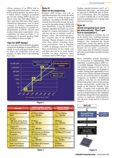
silicon resources of an FPGA lead to
staggering performance gains – while the
fastest general purpose can deliver up to
5 billion MAC/s (multiply-accumulate
per second), leading FPGA devices can
deliver more than 500 billion MAC/s –
that’s more than 100x faster. What’s more,
channelized applications such as those
common to wireless communications
naturally lend themselves to parallel implementations
in FPGAs. Growth rates
in processing speed requirements versus
capabilities are shown in Figure 1 1 . A
comparison of general purpose DSPs
versus FPGAs is shown in Table 1 2 .
Tips for DSP design
Let’s now take a close look at how designers
navigate the challenges of using FPGAs in
design to avoid prolonged design cycles
or reduce the component cost for end
products. It comes down to the following
basic rules.
1
Figure 1
Rule #1
Start at the beginning.
Complex DSP designs start with an
algorithm developer who creates the initial
design based on existing designs and
experience. According to the DSP market
research firm Forward Concepts, the leading
tool for algorithm design is MATLAB
from MathWorks. Using the MATLAB
language, algorithm developers can create
designs in a natural and productive form
and may tap into an immense wealth of
designs, scripts, and engineering knowhow
available only in the MATLAB
language. Though designers can choose
from other options including blocklevel
environments, such as Simulink
or SPW, or languages based on C/C++,
these environments are less widely used
and there may not be as many designs
available for them. Moreover, many
constructs used in DSP designs – such as
looping, repeated structures, and 2- or 3-
dimensional data arrays – are much easier
to represent in MATLAB than in blocklevel
environments. Once the algorithm
is created in MATLAB, it can be readily
shared or partitioned across a design team
and reused over time.
2
Rule #2
Avoid recopying your work
(or alternatively, “Don’t get
lost in translation”).
Once the algorithm is available, the rest
of the design team, including hardware
designers, software developers, and system
designers who integrated the design
components, swings into motion. In the
past, the completed algorithm in MATLAB
became the executable specification,
which meant that the hardware designer
and software developers needed to recreate
the design.
Many embedded systems developers
are accustomed to implementing DSP
algorithms on general purpose DSPs in C
or assembly language. This puts hardware
and software engineers into the role of
translating designs from one language to
another, creating many opportunities for inserting
errors with the attendant debugging
process. To avoid this process altogether,
companies are looking to architectural
synthesis tools that use the MATLAB
M-file as the golden source for downstream
design, automatically synthesizing the
design at the Register Transfer Level
(RTL). Coupled with traditional RTL
synthesis tools that can synthesize RTL to
gate-level implementation, this establishes
an unbroken design flow from algorithmic
creation to hardware implementation.
The top-down design process is shown in
Figure 2.
Function
Industry leading, general
purpose, DSP processor core
Industry leading
platform FPGA
8x8 Multiply Accumulate 4.8 Billion MACps 1 Trillion MACps
(MAC) f clk = 600 MHz f clk = 300 MHz
FIR Filter
– 256 Taps, Linear phase 9.3 Msps 300 Msps
– 16-bit data/coefficients f clk = 600 MHz f clk = 300 MHz
Complex FFT 10 µs 1 µs
– 1024 point, 16-bit data f clk = 600 MHz f clk = 150 MHz
Viterbi decoding 500 channels at 7.95 Kbps 155 Mbps (OC-3 rates)
throughput
for a total of 3.9 Mbps
Reed-Solomon decoding 4.1 Mbps 10 Gbps (OC-192 rates)
throughput f clk = 600 MHz f clk = 85 MHz
Turbo convolutional Six 2 Mbps data streams 5.4 Mbps
decoder throughput (6 iterations) (6 iterations)
Table 1
Figure 2
Embedded Computing Design Summer 2004 / 31