Face Detection and Modeling for Recognition - Biometrics Research ...

More documents

Recommendations

Info

f(u j , v j ) = θ(u j , v j ) = S∑ |∇G σs (u j , v j ) ⊛ Y (u j , v j )| (5.5) s=0 S∑ arg (∇G σs (u j , v j ) ⊛ Y (u j , v j )) , (5.6) s=0 where Y is the luma of the color image I, and G σs is the Gaussian function with zero mean and standard deviation σ s . The largest standard deviation σ S is limited by the distance between eyes and eyebrows where S = 4, and ∇ and ⊛ are the gradient and convolution operators. The gradient magnitude, gradient orientation, eye map [175] and coarse alignment results for the subject in Fig. 5.4(a) are shown in Fig. 5.5. The eye map is an average of a symmetry map [177] and an eye energy map (will be explained in Section 5.3.1). Furthermore, we construct a shadow map of a face image in order to locate eyebrow, nostril, and mouth lines, based on the average value of luminance intensity on a facial skin region (i.e., rectangles shown in Figs. 5.6(a) and 5.6(c)). These feature lines, shown as dark lines in Figs. 5.7(c), are used to adjust corresponding facial components of a semantic graph. Fig. 5.7 shows five examples of coarse alignment. 5.3 Fine Alignment of Semantic Face Graph via Interacting Snakes Fine alignment employs active contours to locally refine facial components of a semantic face graph that is drawn from a 3D generic face model. The 2D projection of 118
(a) (b) (c) (d) Figure 5.5. Boundary map and eye component map for coarse alignment: (a) and (b) are gradient magnitude and orientation, respectively, obtained from multi-scale Gaussian-blurred edge response; (c) an eye map extracted from a face image shown in Fig. 5.4(c); (d) a semantic face graph overlaid on a 3D plot of the eye map; (e) image overlaid with a coarsely aligned face graph. (e) a semantic face graph produces a collection of component boundaries, each of which is described by a closed (or open) active contour. The collection of these active contours, called interacting snakes, interact with each other through a repulsion energy in order to align the general facial topology onto the sensed face images in an iterative fashion. We have studied two competing implementations of active contours for the deformation of interacting snakes: (i) explicit (or parametric) and (ii) implicit contour 119
Page 1 and 2:
Face Detection and Modeling for Rec
Page 3 and 4:
perimental results demonstrate succ
Page 5 and 6:
To my parents; my lovely wife, Pei-
Page 7 and 8:
for providing the range datasets; t
Page 9 and 10:
4 Face Modeling 97 4.1 Modeling Met
Page 11 and 12:
List of Figures 1.1 Applications us
Page 13 and 14:
2.6 A breakdown of face recognition
Page 15 and 16:
4.2 3D triangular-mesh model and it
Page 17 and 18:
5.14 Fine alignment using geodesic
Page 19 and 20:
Chapter 1 Introduction In recent ye
Page 21 and 22:
(a) (b) Figure 1.1. Applications us
Page 23 and 24:
(e) Figure 1.1. (Cont’d). (f) (a)
Page 25 and 26:
esolutions and of poor quality (i.e
Page 27 and 28:
can recognize known faces in carica
Page 29 and 30:
the motivation for studies that att
Page 31 and 32:
(a) Figure 1.10. Similarity of fron
Page 33 and 34:
verify the face present in an image
Page 35 and 36:
17 Figure 1.12. System diagram of o
Page 37 and 38:
algorithm can also provide geometri
Page 39 and 40:
commercial parametric face modeling
Page 41 and 42:
1.5.1 Face Alignment Using 2.5D Sna
Page 43 and 44:
1.5.3 Face Alignment Using Interact
Page 45 and 46:
Using merely low-level features (e.
Page 47 and 48:
such as eyes, mouth and face bounda
Page 49 and 50:
can be applied to a 3D face model w
Page 51 and 52:
Chapter 2 Literature Review We firs
Page 53 and 54:
mation theory, geometrical modeling
Page 55 and 56:
(e) (f) (g) (h) (i) (j) (k) (l) Fig
Page 57 and 58:
esult in different recognition appr
Page 59 and 60:
(a) (b) (c) Figure 2.2. Examples of
Page 61 and 62:
(a) (b) (c) (d) Figure 2.4. Interna
Page 63 and 64:
Figure 2.6. A breakdown of face rec
Page 65 and 66:
2.3 Face Modeling Face modeling pla
Page 67 and 68:
An advanced modeling approach which
Page 69 and 70:
tionals to minimize, implementation
Page 71 and 72:
are listed in Table 2.2. All of the
Page 73 and 74:
low-level features can provide mean
Page 75 and 76:
holistic 2D and geometrical 3D feat
Page 77 and 78:
size) to generate potential face ca
Page 79 and 80:
oundary. A face score is computed f
Page 81 and 82:
normalized red-green (r-g) space [1
Page 83 and 84:
(a) (b) Figure 3.3. The Y C b C r c
Page 85 and 86: (a) Figure 3.5. 2D projections of t
Page 87 and 88: 3.3 Localization of Facial Features
Page 89 and 90: (a) (b) (c) Figure 3.9. Constructio
Page 91 and 92: The eye map from the chroma is enha
Page 93 and 94: mouth is performed within the face
Page 95 and 96: Figure 3.12. Computation of face bo
Page 97 and 98: center, and lengths of major and mi
Page 99 and 100: segment. The other term favors an u
Page 101 and 102: (a) (b) (c) (d) (e) Figure 3.15. Fa
Page 103 and 104: (a) (b) (c) (d) (e) Figure 3.18. Fa
Page 105 and 106: The number of false positives is al
Page 107 and 108: (a) (b) (c) (d) Figure 3.20. Face d
Page 109 and 110: Figure 3.22. Face detection results
Page 111 and 112: Figure 3.22. (Cont’d). 93
Page 113 and 114: 3.5 Summary We have presented a fac
Page 115 and 116: Chapter 4 Face Modeling We first in
Page 117 and 118: and nose in frontal views), and bec
Page 119 and 120: 4.3 Facial Measurements Facial meas
Page 121 and 122: 4.4 Model Construction Our face mod
Page 123 and 124: a feature-dependent decay factor. F
Page 125 and 126: is to find appropriate external ene
Page 127 and 128: (a) (b) (d) (e) (f) Figure 4.11. Te
Page 129 and 130: Chapter 5 Semantic Face Recognition
Page 131 and 132: (a) (b) (c) Figure 5.1. Semantic fa
Page 133 and 134: of Fourier series truncation. In ad
Page 135: ponent color. The semantic facial s
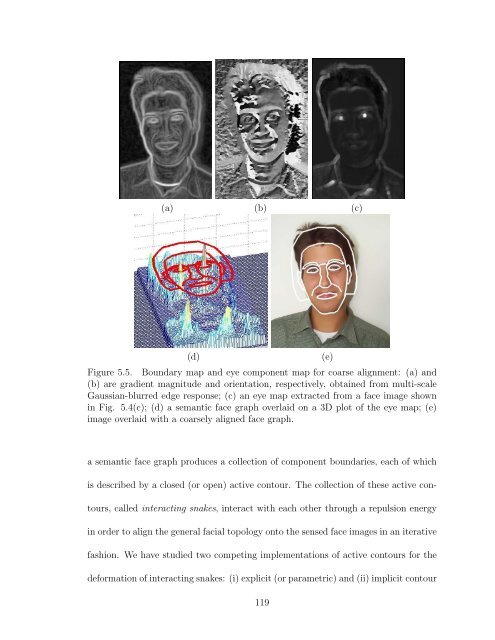
Page 139 and 140: (a) (b) (c) (d) Figure 5.7. Coarse
Page 141 and 142: In the Baysian framework, given an
Page 143 and 144: edge map; hence it requires a clean
Page 145 and 146: shows examples of mouth energies. F
Page 147 and 148: [ ( ∂Φ ∂t =∇Φ µ 1 div(g
Page 149 and 150: (a) (b) (c) (d) (e) (f) Figure 5.14
Page 151 and 152: y the reliability of component matc
Page 153 and 154: tation, face size, and lighting con
Page 155 and 156: (a) (b) (c) (d) Figure 5.18. Exampl
Page 157 and 158: (a) (b) (c) (d) (e) (f) (g) (h) (i)
Page 159 and 160: (a) (b) (c) (d) (e) (f) (g) Figure
Page 161 and 162: 5.6 Summary For overcoming variatio
Page 163 and 164: such vision-based systems are (i) d
Page 165 and 166: 6.2 Future Directions Based on the
Page 167 and 168: (a) (b) (c) (d) Figure 6.2. An exam
Page 169 and 170: • Non-frontal training views: Acc
Page 171 and 172: Appendices
Page 173 and 174: ⎡ ⎤ ⎡ ⎤ ⎡ ⎤ ⎡ ⎤ Y
Page 175 and 176: and are shown as blue-dashed lines
Page 177 and 178: adius of a cluster ‘i’ w.r.t. a
Page 179 and 180: Appendix C Image Processing Templat
Page 181 and 182: considering pixel classes as voxel
Page 183 and 184: gray8imageA(120,120) = 200; // Asse
Page 185 and 186: Bibliography [1] Visionics Corporat
Page 187 and 188:
[32] L. Wiskott, J.M. Fellous, N. K
Page 189 and 190:
[59] M. Grudin, “On internal repr
Page 191 and 192:
[84] M. Abdel-Mottaleb and A. Elgam
Page 193 and 194:
[113] B. Kim and P. Burger, “Dept
Page 195 and 196:
[141] M.D. Adams and F. Kossentini,
Page 197 and 198:
[169] P.T. Jackway and M. Deriche,
show all

Face Detection and Modeling for Recognition - Biometrics Research ...

Create successful ePaper yourself

Delete template?

Save as template?