Aerial and Acoustic Surveys for Mackerel - BioSonics, Inc

Equally good progress has been made with the identification of fish without swim-bladders (see Sections 3.2 and 3.3
below). A number of algorithm development approaches have been pursued: one incorporating many frequencies as
part of a frequency response based algorithm and one based on a triple frequency dB difference algorithm. Both have
now been applied to mackerel. Two participants have conducted dedicated research cruises to target mackerel and there
is, therefore, a large dataset which is available to verify these algorithms in year three.
It seems as though the frequency dependence of fish with swim-bladders is likely to be too invariant at most frequencies
(38–200 kHz) to be able to develop an algorithm for the differentiation amongst these species. Efforts will therefore be
concentrated on less common lower frequencies (12–18 kHz) which have shown to be possibly useful for size
discrimination. Effort will also be put into analysis of extracted parameters at any one frequency to assist in the
identification process.
At each step of algorithm development for a particular species, combinations of algorithms have been considered. In
some cases, e.g., mackerel, the algorithms are part of a suite which aims to identify other targets also. In combination
with noise and plankton filters, there are good prospects for providing algorithms which encompass many aspects of the
identification process.
3.2 IMR mackerel identification algorithm
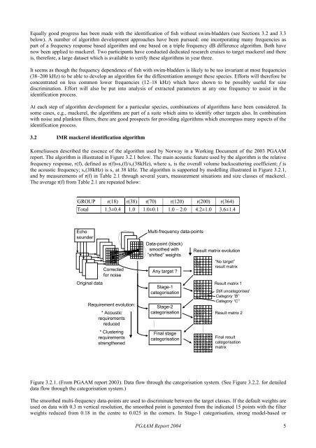
Korneliussen described the essence of the algorithm used by Norway in a Working Document of the 2003 PGAAM
report. The algorithm is illustrated in Figure 3.2.1 below. The main acoustic feature used by the algorithm is the relative
frequency response, r(f), defined as r(f)≡s v (f)/s v (38kHz), where s v is the overall volume backscattering coefficient; f is
the acoustic frequency; s v (38kHz) is s v at 38 kHz. The algorithm is supported by modelling illustrated in Figure 3.2.1,
and by measurements of r(f) in Table 2.1 through several years, measurement situations and size classes of mackerel.
The average r(f) from Table 2.1 are repeated below:
GROUP r(18) r(38) r(70) r(120) r(200) r(364)
Total 1.3±0.4 1.0 1.0±0.1 1.0 – 2.0 4.2±1.0 3.6±1.4
Echo
sounder
Original data
Corrected
for noise
Requirement evolution:
* Acoustic
requirements
reduced
* Clustering
requirements
strengthened
Multi-frequency data-points
Data-point (black)
smoothed with
”shifted” weights
Any target ?
Stage-1
categorisation
Stage-2
categorisation
Final stage
categorisation
Result matrix evolution
N
N
N
N
N
N
N
N
C
N
N
N
N
C
C
N
N
N
N
C
C
C
N
N
A
N
N
A
N
N
C
A
A
N
N
C
C
C
N
N
A
A
A
N
N
A
A
A
A
N
N
A
A
A
A
N
N
C
B
A
A
B
B
A
A
A
A
B
B
B
B
B
A
A
D
D
B
B
A
D
B
A
A
D
D
D
B
“No target”
result matrix
Result matrix 1
Still uncategorised
Category “B”
Category “C”
Result matrix 2
Final result
categorisation
matrix
Figure 3.2.1. (From PGAAM report 2003). Data flow through the categorisation system. (See Figure 3.2.2. for detailed
data flow through the categorisation system.)
The smoothed multi-frequency data-points are used to discriminate between the target classes. If the default weights are
used on data with 0.3 m vertical resolution, the smoothed point is generated from the indicated 15 points with the filter
weights reduced from 0.18 in the centre to 0.025 in the corners. In Stage-1 categorisation, strong model-based or
PGAAM Report 2004 5