"Top Incomes in the Long Run of History" with Tony Atkinson and

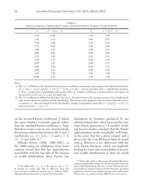
14Journal of Economic Literature, Vol. XLIX (March 2011)Table 3Pareto-Lorenz α Coefficients versus Inverted-Pareto-Lorenz β Coefficientsα β = α/(α − 1) β α = β/(β − 1)1.10 11.00 1.50 3.001.30 4.33 1.60 2.671.50 3.00 1.70 2.431.70 2.43 1.80 2.251.90 2.11 1.90 2.112.00 2.00 2.00 2.002.10 1.91 2.10 1.912.30 1.77 2.20 1.832.50 1.67 2.30 1.773.00 1.50 2.40 1.714.00 1.33 2.50 1.675.00 1.25 3.00 1.5010.00 1.11 3.50 1.40Notes:(1) The “α” coefficient is the standard Pareto-Lorenz coefficient commonly used in power-law distribution formulas:1−F(y) = (A/y) α and f(y) = αA α /y 1+α (A>0, α>1, f(y) = density function, F(y) = distribution function,1−F(y) = proportion of population with income above y). A higher coefficient α means a faster convergence ofthe density toward zero, i.e., a less fat upper tail.(2) The “β” coefficient is defined as the ratio y*(y)/y, i.e., the ratio between the average income y*(y) of individualswith income above threshold y and the threshold y. The characteristic property of power laws is that this ratio isa constant, i.e., does not depend on the threshold y. Simple computations show that β = y*(y)/y = α/(α−1),and conversely α = β/(β−1).on the inverted Pareto coefficient β (whichhas more intuitive economic appeal) ratherthan the standard Pareto coefficient α. Notethat there exists a one-to-one, monotonicallydecreasing relationship between the α and βcoefficients, i.e., β = α/(α − 1) and α = β/(β − 1) (see table 3). 11Vilfredo Pareto (1896, 1896–1897), inthe 1890s using tax tabulations from Swisscantons, found that this law approximatesremarkably well the top tails of the incomeor wealth distributions. Since Pareto, raw11 Put differently, (β − 1) is the inverse of (α − 1).It should be noted that this is different from theinverse-Pareto coefficient used by Lee C. Soltow (1969),although this too increases as the tail becomes fatter.tabulations by brackets produced by taxadministrations have often been used to estimatePareto parameters. 12 A number of thetop income studies conclude that the Paretoapproximation works remarkably well today,in the sense that for a given country and agiven year, the β coefficient is fairly invariantwith y. However a key difference with theearly Pareto literature, which was implicitlylooking for some universal stability of incomeand wealth distributions, is that our much12 There also exists a voluminous theoretical literaturetrying to explain why Pareto laws fit the top tails of incomeand wealth distributions. We survey some of these theoreticalmodels in section 5 below. Pareto laws have also beenapplied in several areas outside income and wealth distribution(see, e.g., Xavier Gabaix 2009 for a recent survey).