- Page 2 and 3:
Library of Congress Cataloging-in-P
- Page 7 and 8:
III. Statistical Considerations •
- Page 9 and 10:
IV. Further Generalizations — 183
- Page 11:
Appendix 6A:Unbiased Estimation of
- Page 14 and 15:
2 Monte Carlo Particle Transport Me
- Page 17 and 18:
Chapter 2INTRODUCTIONWhen we starte
- Page 19 and 20:
thus,As it is proved" — and is so
- Page 21 and 22:
9B. THE PROBABILITY MIXING METHODTh
- Page 23 and 24:
11It is easy to prove 15by summing
- Page 25 and 26:
13but the most probable values:x, =
- Page 27 and 28:
ISand give a random sign (by the us
- Page 30 and 31:
18 Monte Carlo Particle Transport M
- Page 32 and 33:
20 Monte Carlo Particle Transport M
- Page 34 and 35:
22 Monte Carlo Particle Transport M
- Page 36 and 37:
24 Monte Carlo Particle Transport M
- Page 38 and 39:
26 Monte Carlo Particle Transport M
- Page 40 and 41:
28 Monte Carlo Particle Transport M
- Page 42 and 43:
30 Monte Carlo Particle Transport M
- Page 44 and 45:
">3
- Page 46 and 47:
34 Monte Carlo Particle Transport M
- Page 48 and 49:
36 Monte Carlo Particle Transport M
- Page 50 and 51:
38 Monte Carlo Particle Transport M
- Page 52 and 53: 40 Monte Carlo Particle Transport M
- Page 54 and 55: 42 Monte Carlo Particle Transport M
- Page 56 and 57: 44 Monte Carlo Particle Transport M
- Page 58 and 59: 46 Monte Carlo Particle Transport M
- Page 60 and 61: 48 Monte Carlo Particle Transport M
- Page 62 and 63: 50 Monte Carlo Particle Transport M
- Page 64 and 65: 52 Monte Carlo Particle Transport M
- Page 66 and 67: 54 Monte Carlo Particle Transport M
- Page 68 and 69: 56 Monte Carlo Particle Transport M
- Page 70 and 71: 58 Monte Carlo Particle Transport M
- Page 72 and 73: 60 Monte Carlo Particle Transport M
- Page 74 and 75: 62 Monte Carlo Particle Transport M
- Page 76 and 77: 64 Monte Carlo Particle Transport M
- Page 78 and 79: 66 Monte Carlo Particle Transport M
- Page 80 and 81: 68 Monte Carlo Particle Transport M
- Page 82 and 83: 70 Monte Carlo Particle Transport M
- Page 84 and 85: 72 Monte Carlo Particle Transport M
- Page 86 and 87: 74 Monte Carlo Particle Transport M
- Page 88 and 89: 76 Monte Carlo Particle Transport M
- Page 90 and 91: 78 Monte Carlo Particle Transport M
- Page 92 and 93: 80 Monte Carlo Particle Transport M
- Page 94 and 95: 82 Monte Carlo Particle Transport M
- Page 96 and 97: 84 Monte Carlo Particle Transport M
- Page 98 and 99: 86 Monte Carlo Particle Transport M
- Page 100 and 101: 88 Monte Carlo Particle Transport M
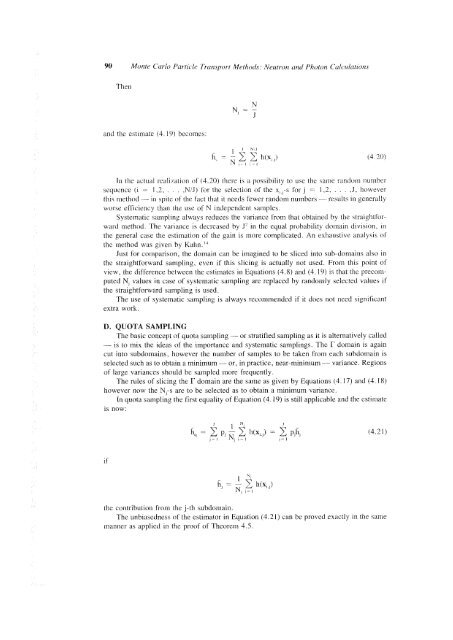
- Page 104 and 105: 92 Monte Carlo Particle Transport M
- Page 106 and 107: 94 Monte Carlo Particle Transport M
- Page 108 and 109: 96 Monte Carlo Particle Transport M
- Page 110 and 111: 98 Monte Carlo Particle Transport M
- Page 112 and 113: 100 Monte Carlo Panicle Transport M
- Page 114 and 115: 102 Monte Carlo Particle Transport
- Page 116 and 117: 104 Monte Carlo Particle Transport
- Page 118 and 119: 106 Monte Carlo Particle Transport
- Page 120 and 121: 108 Monte Carlo Particle Transport
- Page 122 and 123: 110 Monte Carlo Particle Transport
- Page 124 and 125: 112 Monte Carlo Particle Transport
- Page 126 and 127: 114 Monte Carlo Particle Transport
- Page 128 and 129: 116 Monte Carlo Particle Transport
- Page 130 and 131: 118 Monte Carlo Particle Transport
- Page 132 and 133: 120 Monte Carlo Particle Transport
- Page 134 and 135: 122 Monte Carlo Particle Transport
- Page 136 and 137: 124 Monte Carlo Particle Transport
- Page 138 and 139: 126 Monte Carlo Particle Transport
- Page 140 and 141: 128 Monte Carlo Particle Transport
- Page 142 and 143: 130 Monte Carlo Particle Transport
- Page 144 and 145: 132 Monte Carlo Particle Transport
- Page 146 and 147: 134 Monte Carlo Particle Transport
- Page 148 and 149: 136 Monte Carlo Particle Transport
- Page 150 and 151: 138 Monte Carlo Particle Transport
- Page 152 and 153:
140 Monte Carlo Particle Transport
- Page 154 and 155:
142 Monte Carlo Particle Transport
- Page 156 and 157:
144 Monte Carlo Particle Transport
- Page 158 and 159:
146 Monte Carlo Particle Transport
- Page 160 and 161:
148 Monte Carlo Particle Transport
- Page 162 and 163:
150 Monte Carlo Particle Transport
- Page 164 and 165:
152 Monte Carlo Particle Transport
- Page 166 and 167:
154 Monte Carlo Particle Transport
- Page 168 and 169:
156 Monte Carlo Particle Transport
- Page 170 and 171:
158 Monte Carlo Particle Transport
- Page 172 and 173:
160 Monte Carlo Particle Transport
- Page 174 and 175:
162 Monte Carlo Particle Transport
- Page 176 and 177:
164 Monte Carlo Particle Transport
- Page 178 and 179:
166 Monte Carlo Particle Transport
- Page 180 and 181:
168 Monte Carlo Particle Transport
- Page 182 and 183:
170 Monte Carlo Particle Transport
- Page 184 and 185:
172 Monte Carlo Particle Transport
- Page 186 and 187:
174 Monte Carlo Particle Transport
- Page 188 and 189:
176 Monte Carlo Particle Transport
- Page 190 and 191:
178 Monte Carlo Particle Transport
- Page 192 and 193:
180 Monte Carlo Particle Transport
- Page 194 and 195:
182 Monte Carlo Particle Transport
- Page 196 and 197:
184 Monte Carlo Particle Transport
- Page 198 and 199:
186 Monte Carlo Particle Transport
- Page 200 and 201:
188 Monte Carlo Particle Transport
- Page 202 and 203:
190 Monte Carlo Particle Transport
- Page 204 and 205:
192 Monte Carlo Particle Transport
- Page 206 and 207:
194 Monte Carlo Particle Transport
- Page 208 and 209:
196 Monte Carlo Particle Transport
- Page 210 and 211:
198 Monte Carlo Particle Transport
- Page 212 and 213:
200 Monte Carlo Particle Transport
- Page 214 and 215:
202 Monte Carlo Particle Transport
- Page 216 and 217:
204 Monte Carlo Particle Transport
- Page 218 and 219:
206 Monte Carlo Particle Transport
- Page 220 and 221:
208 Monte Carlo Particle Transport
- Page 222 and 223:
210 Monte Carlo Particle Transport
- Page 224 and 225:
212 Monte Carlo Particle Transport
- Page 226 and 227:
214 Monte Carlo Particle Transport
- Page 228 and 229:
216 Monte Carlo Particle Transport
- Page 230 and 231:
218 Monte Carlo Particle Transport
- Page 232 and 233:
220 Monte Carlo Particle Transport
- Page 234 and 235:
222 Monte Carlo Particle Transport
- Page 236 and 237:
224 Monte Carlo Particle Transport
- Page 238 and 239:
226 Monte Carlo Particle Transport
- Page 240 and 241:
228 Monte Carlo Particle Transport
- Page 242 and 243:
230 Monte Carlo Particle Transport
- Page 244 and 245:
232 Monte Carlo Particle Transport
- Page 246 and 247:
234 Monte Carlo Particle Transport
- Page 248 and 249:
236 Monte Carlo Particle Transport
- Page 250 and 251:
238 Monte Carlo Particle Transport
- Page 252 and 253:
240 Monte Carlo Particle Transport
- Page 254 and 255:
242 Monte Carlo Particle Transport
- Page 256 and 257:
244 Monte Carlo Particle Transport
- Page 258 and 259:
246 Monte Carlo Particle Transport
- Page 260 and 261:
248 Monte Carlo Particle Transport
- Page 262 and 263:
25!) Monte Carlo Particle Transport
- Page 264 and 265:
252 Monte Carlo Particle Transport
- Page 266 and 267:
254 Monte Carlo Particle Transport
- Page 268 and 269:
256 Monte Carlo Particle Transport
- Page 270 and 271:
258 Monte Carlo Particle Transport
- Page 272 and 273:
260 Monte Carlo Particle Transport
- Page 274 and 275:
262 Monte Carlo Particle Transport
- Page 276 and 277:
264 Monte Carlo Particle Transport
- Page 278 and 279:
266 Monte Carlo Particle Transport
- Page 280 and 281:
268 Monte Carlo Particle Transport
- Page 282 and 283:
270 Monte Carlo Particle Transport
- Page 284 and 285:
272 Monte Carlo Particle Transport
- Page 286 and 287:
274 Monte Carlo Particle Transport
- Page 288 and 289:
276 Monte Carlo Particle Transport
- Page 290 and 291:
278 Monte Carlo Particle Transport
- Page 292 and 293:
280 Monte Carlo Particle Transport
- Page 294 and 295:
282 Monte Carlo Particle Transport
- Page 296 and 297:
284 Monte Carlo Particle Transport
- Page 298 and 299:
286 Monte Carlo Particle Transport
- Page 300 and 301:
288 Monte Carlo Particle Transport
- Page 302 and 303:
290 Monte Carlo Particle Transport
- Page 304 and 305:
292 Monte Carlo Particle Transport
- Page 306 and 307:
294 Monte Carlo Particle Transport
- Page 308 and 309:
296 Monte Carlo Particle Transport
- Page 310 and 311:
298 Monte Carlo Particle Transport
- Page 312 and 313:
300 Monte Carlo Particle Transport
- Page 314 and 315:
302 Monte Carlo Particle Transport
- Page 317 and 318:
305Chapter 6SPECIAL GAMESIn the maj
- Page 319 and 320:
3©7A. CORRELATED MOMENT EQUATIONSI
- Page 321 and 322:
309Equation (6.1) will be referred
- Page 323 and 324:
311The second moment of the score d
- Page 325 and 326:
313andC S(P',P")/C S(P',P") = y(P',
- Page 327 and 328:
315introduced in Equation (6.1) for
- Page 329 and 330:
317andL„(P 0,P;,...,Pi + 1) = L n
- Page 331 and 332:
319whereB„(P„,P; P:, ,) = A*(P
- Page 333 and 334:
E. EXAMPLES AND SPECIAL TECHNIQUESL
- Page 335 and 336:
323The weight factors associated wi
- Page 337 and 338:
325It is seen from Equation (6.37)
- Page 339 and 340:
327G. PARAMETRIC PERTURBATIONS: INT
- Page 341 and 342:
129Hall 31 gave a constructive deri
- Page 343 and 344:
331kernels, which remain unchanged
- Page 345 and 346:
333and from Equation (6.51)w';,,(i)
- Page 347 and 348:
335According to Equations (6,55) th
- Page 349 and 350:
337Minimization is performed by set
- Page 351 and 352:
339and letdsdaLet us consider a cor
- Page 353 and 354:
341whereis the length of the flight
- Page 355 and 356:
and from Equation (6.79)I / ds \ 2
- Page 357 and 358:
345Let us assume that we are intere
- Page 359 and 360:
347Introduction of this factor also
- Page 361 and 362:
3492. Let i|/ n (P) denote the solu
- Page 363 and 364:
3SJNow, if ( "> > 0, then k = i an
- Page 365 and 366:
353andk„ = S l "VS'" •" (6. if;
- Page 367 and 368:
3SSLet k„ denote the normalizatio
- Page 369 and 370:
3572. It is then proved that with t
- Page 371 and 372:
and start new histories until N new
- Page 373 and 374:
361The application of source iterat
- Page 375 and 376:
363we haveD 2 [k] = < 2 (k, - k,) )
- Page 377 and 378:
365neutron density, S 0 for every
- Page 379 and 380:
367if the same relation holds for t
- Page 381 and 382:
369Then the multiplication factors
- Page 383 and 384:
371in the unperturbed system, the w
- Page 385 and 386:
373The perturbation of the effectiv
- Page 387 and 388:
375where P" = (r',E'). Multiplying
- Page 389 and 390:
377iterate of the derivative of the
- Page 391 and 392:
579where P* = (r*,w*,E) = (r*,E*).
- Page 393 and 394:
381This estimator, unlike f, in Equ
- Page 395 and 396:
383tends to some stable attracting
- Page 397 and 398:
3§SIo the case of the next-event e
- Page 399 and 400:
387LDFIGURE 6.1.Geometry in scoring
- Page 401 and 402:
389Let us denoteThen Equation (6.18
- Page 403 and 404:
391is to be increased in order to o
- Page 405 and 406:
393Now, since bl(P) = g(P) is bound
- Page 407 and 408:
395is scored at every collision wit
- Page 409 and 410:
397and its expectation isR — R 1n
- Page 411 and 412:
3994. If O > 0 m, then the particle
- Page 413 and 414:
401plays a distinguished role), and
- Page 415 and 416:
403Theorem 6.7 — If x and s denot
- Page 417 and 418:
this a priori information, the best
- Page 419 and 420:
40?Thus, the bias introduced into t
- Page 421 and 422:
409In view of Equation (6.226) and
- Page 423 and 424:
41.1This means that if we use the k
- Page 425 and 426:
413Then the whole-sample and rare-s
- Page 427 and 428:
41.5According to the results of Sec
- Page 429 and 430:
41?(Note that vD 2 [|i|v] is indepe
- Page 431 and 432:
419withkOn the other hand, § is an
- Page 433 and 434:
421Thus, the expected ratio reads
- Page 435 and 436:
423St follows from Equations (6.265
- Page 437 and 438:
425Wc start from the observation th
- Page 439 and 440:
427Nowi'6.77K)kj„,and therefore(V
- Page 441 and 442:
42*3Similarly, for the fourth momen
- Page 443 and 444:
43 sOn the other hand, multiplying
- Page 445 and 446:
43.¾This will be proven in the lem
- Page 447 and 448:
435ThenT.m = EJ.Iy.y.Rjeyiy,,,and s
- Page 449 and 450:
6. Brown. F. B. and Martin, W. R.,
- Page 451:
67. Rief, H. and Fioretti, A., Mont
- Page 454 and 455:
442 Monte Carlo Particle Transport
- Page 456 and 457:
444 Monte Carlo Particle Transport
- Page 458 and 459:
446 Monte Carlo Particle Transport
- Page 460 and 461:
448 Monte Carlo Particle Transport
- Page 462 and 463:
450 Monte Carlo Particle Transport
- Page 464 and 465:
452 Monte Carlo Particle Transport
- Page 466 and 467:
454 Monte Carlo Particle Transport
- Page 468 and 469:
456 Monte Carlo Particle Transport
- Page 470 and 471:
458 Monte Carlo Particle Transport
- Page 472 and 473:
460 Monte Carlo Particle Transport
- Page 474 and 475:
462 Monte Carlo Particle Transport
- Page 476 and 477:
464 Monte Carlo Particle Transport
- Page 478 and 479:
466 Monte Carlo Particle Transport
- Page 480 and 481:
468 Monte Carlo Particle Transport
- Page 482 and 483:
Q = iy.M 2 2 (1/T, - 1/1,..,)/1, £
- Page 484 and 485:
472 Monte Carlo Particle Transport
- Page 486 and 487:
474 Monte Carlo Particle Transport
- Page 488 and 489:
476 Monte Carlo Particle Transport
- Page 490 and 491:
478 Monte Carlo Particle Transport
- Page 492 and 493:
48© Monte Carlo Particle Transport
- Page 494 and 495:
482 Monte Carlo Particle Transport
- Page 496 and 497:
484 Monte Carlo Panicle Transport M
- Page 498 and 499:
486 Monte Carlo Panicle Transport M
- Page 500 and 501:
488 Monte Carlo Particle Transport
- Page 502 and 503:
490 Monte Carlo Particle Transport
- Page 504 and 505:
492 Monte Carlo Particle Transport
- Page 506 and 507:
494 Monte Carlo Particle Transport
- Page 508 and 509:
496 Monte Carlo Particle Transport
- Page 510 and 511:
498 Monte Carlo Particle Transport
- Page 512 and 513:
500 Monte Carlo Particle Transport
- Page 514 and 515:
502 Monte Carlo Particle Transport
- Page 516 and 517:
504 Monte Carlo Particle Transport
- Page 518 and 519:
a ( X506 Monte Carlo Particle Trans
- Page 520 and 521:
508 Monte Carlo Particle Transport
- Page 522 and 523:
510 Monte Carlo Particle Transport
- Page 525 and 526:
513INDEXAAbsorptiondefined, 25photo
- Page 527 and 528:
515score probability in general tim
- Page 529:
517path stretching, 447—455splitt


