The Limits of Mathematics and NP Estimation in ... - Chichilnisky

More documents

Recommendations

Info

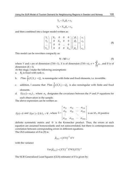
Using the SUR Model of Tourism Demand for Neighbouring Regions in Sweden and Norway 105Y X e2 2 2 2Y X em m m mand then combined into a larger model written as:Y1 X1 0 0 0 1 e1 Y2 0 X2 0 0 2 e2 ... 0 0 ... 0 ... ... Y m 0 0 0 X m m e mThis model can be rewritten compactly as:(8)YX Be(9)where Y and e are of dimension (TM 1), X is of dimension (TM n), n =dimension (K 1).At this stage, I make the following assumptions:a. X i is fixed with rank n i .M nii1, and B is ofb. P lim1 ('XX i i )T Q ii is nonsingular with finite and fixed elements, i.e. invertible.c. addition, I assume that Plimd.1 ('XX i j ) Q ij is also nonsingular with finite and fixedTelements.,Eee ( i i) ijIT, where ij designates the covariance between the i th and j th equations foreach observation in the sample.The above expression can be written as: 11 12 1MEe () 0and ,21 22 2MEee ( ) IT, where is an M M positiveM1 M2 MMdefinite symmetric matrix and is the Kronecker product. Thus, the errors at eachequation are assumed homoscedastic and not autocorrelated, but there is contemporaneouscorrelation between corresponding errors in different equations.The OLS estimator of B in (9) is:with the variance 1ˆOLS XX XY Var( ˆ ) X X X X( X X)OLS 1 1 The SUR Generalized Least Squares (GLS) estimator of B is given by:
106Advances in Econometrics - Theory and Applicationsand the variance is given by: 1ˆ 1 1GLS ( T ) ( T )X I X X I Y ˆ ( 1) 1GLS TV X I XHowever, the system of the five equations for Sweden and Norway are as follows:Y it= i + S i + XitB i+ Y it-q iq + e ,it i 1, 2, 5 q 1, 2, 12(10)where Y it is a T 1 vector of observations on the dependent variable, e it is a T 1 vector ofrandom errors with E(e t ) = 0 , and S i are monthly dummy variables that take valuesbetween 1 and 11 (the twelfth month is the base). X it is a T nimatrix of observations on n inonstochastic explanatory variables, and B i is an ni 1 dimensional vector of unknownlocation parameters. T is the number of observations per equation, and n i is the number ofrows in the vector B i . iq is a parameter vector associated with the lagged dependentvariable for the respective equation.The dependent variables Y i are the natural logarithms of the number of monthly visitorsfrom Denmark, the UK, Switzerland, Japan, and the US to either Sweden or Norway. Thematrix X i is the natural logarithm of three vectors that contains monthly information aboutthe CPI in Sweden (or Norway), the exchange rate (Ex) in Sweden (or Norway), and relativeprice (Rp) for Sweden (or Norway) with respect to each of the abovementioned countries.Another objective of this study is to test for the existence of any contemporaneouscorrelation between the equations. If such correlation exists and is statistically significant,then least squares applied separately to each equation are not efficient and there is need toemploy another estimation method that is more efficient.The SUR estimators utilize the information present in the cross regression (or equations)error correlation. In this chapter, we estimated the model in Equation (10) by using the OLSmethod for each equation separately to achieve the best specification of each equation. Wethen estimate the whole system using ISUR, see Tables 2 and 3. The ISUR techniqueprovides parameter estimates that converge to unique maximum likelihood parameterestimates and take into account any possible contemporaneous correlation between theequations.To test whether the estimated correlation between these equations is statistically significant,we apply Breusch and Pagan’s (1980) LM statistic. If we denote the covariances between thedifferent equations as 12 , 13 … 45 , the null hypothesis is:H 0 : 12 = 13 . . . = 45 = 0, against the alternative hypothesis,H 1 : at least one covariance is nonzero.In our three equations, the test statistic is: = N(r 2 12 + r 2 13 +…r 2 45), where r 2 ij is the squared correlation,r 2 ij = 2 ij / ii jj .Under H 0 , has an asymptotic 2 distribution with five degrees of freedom. I may reject H 0for a value of greater than the critical value from a 2 (45) distribution (i.e. with 45 degrees offreedom) for a specified significance level. In this study, the calculated 2 value for Sweden
Page 2 and 3:
ADVANCES INECONOMETRICS - THEORYAND
Page 4:
free online editions of InTechBooks
Page 8 and 9:
PrefaceEconometrics is a (sub)disci
Page 10:
PrefaceIXLastly, I would like to th
Page 14:
10The Limits of Mathematicsand NP E
Page 17 and 18:
6 Advances in Econometrics - Theory
Page 19 and 20:
8 Advances in Econometrics - Theory
Page 21 and 22:
10 Advances in Econometrics - Theor
Page 23 and 24:
Page 25 and 26:
Page 27:
Page 32 and 33:
Instrument Generating Functionand A
Page 34 and 35:
Page 36 and 37:
Page 38 and 39:
Page 41 and 42:
30Advances in Econometrics - Theory
Page 44:
Recent Developments in SeasonalVola
Page 47 and 48:
Page 49 and 50:
Page 51 and 52:
Page 53 and 54:
Page 55 and 56:
Page 58 and 59:
The Impact of Government-Sponsored
Page 60 and 61:
The Impact of Government-SponsoredT
Page 62 and 63:
Page 64 and 65:
Page 66 and 67: The Impact of Government-SponsoredT
Page 90 and 91: Returns to Education and Experience
Page 108 and 109: Using the SUR Model of Tourism Dema
show all

The Limits of Mathematics and NP Estimation in ... - Chichilnisky

You also want an ePaper? Increase the reach of your titles

Delete template?

Save as template?