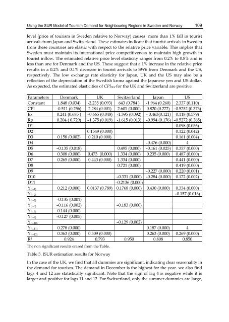
Us<strong>in</strong>g the SUR Model <strong>of</strong> Tourism Dem<strong>and</strong> for Neighbour<strong>in</strong>g Regions <strong>in</strong> Sweden <strong>and</strong> Norway 109level (price <strong>of</strong> tourism <strong>in</strong> Sweden relative to Norway) causes more than 1% fall <strong>in</strong> touristarrivals from Japan <strong>and</strong> Switzerl<strong>and</strong>. <strong>The</strong>se estimates <strong>in</strong>dicate that tourist arrivals <strong>in</strong> Swedenfrom these countries are elastic with respect to the relative price variable. This implies thatSweden must ma<strong>in</strong>ta<strong>in</strong> its <strong>in</strong>ternational price competitiveness to ma<strong>in</strong>ta<strong>in</strong> high growth <strong>in</strong>tourist <strong>in</strong>flow. <strong>The</strong> estimated relative price level elasticity ranges from 0.2% to 0.8% <strong>and</strong> isless than one for Denmark <strong>and</strong> the US. <strong>The</strong>se suggest that a 1% <strong>in</strong>crease <strong>in</strong> the relative priceresults <strong>in</strong> a 0.2% <strong>and</strong> 0.1% decrease <strong>in</strong> tourist arrivals to SW6 from Denmark <strong>and</strong> the US,respectively. <strong>The</strong> low exchange rate elasticity for Japan, UK <strong>and</strong> the US may also be areflection <strong>of</strong> the depreciation <strong>of</strong> the Swedish krona aga<strong>in</strong>st the Japanese yen <strong>and</strong> US dollar.As expected, the estimated elasticities <strong>of</strong> CPI SW for the UK <strong>and</strong> Switzerl<strong>and</strong> are positive.Parameters Denmark UK Switzerl<strong>and</strong> Japan USConstant 1.848 (0.034) -2.235 (0.093) 643 (0.784 ) -1.964 (0.260) 2.337 (0.110)CPI -0.511 (0.256) 2.284 (0.001) 2.601 (0.000) 0.820 (0.272) –0.5252 (0.373)Ex 0.241 (0.685 ) –0.665 (0.048) -1.395 (0.092) – 0.463(0.121) 0.118 (0.579)Rp 0.204 ( 0.729) –1.375 (0.019) -1.615 (0.013) –0.994 (0.176) –0.5272 (0.365)D1 0.098 (0.056)D2 0.1549 (0.000) 0.122 (0.042)D3 0.158 (0.002) 0.210 (0.000) 0.161 (0.004)D4 –0.476 (0.000) 4D5 –0.135 (0.018) 0.495 (0.000) –0.161 (0.025) 0.357 (0.000)D6 0.308 (0.000) 0.473 (0.000) 1.334 (0.000) 0.235 (0.000) 0.487 (0.000)D7 0.265 (0.000) 0.443 (0.000) 1.334 (0.000) 0.441 (0.000)D8 0.721 (0.000) 0.419 (0.000)D9 –0.227 (0.000) 0.220 (0.001)D10 –0.331 (0.000) –0.284 (0.000) 0.172 (0.002)D11 –0.2136 (0.000)Y (t–1) 0.212 (0.000) 0.0137 (0.789) 0.1768 (0.000) 0.430 (0.000) 0.334 (0.000)Y (t–2) –0.157 (0.016)Y (t–3) –0.135 (0.001)Y (t–6) –0.116 (0.002) –0.183 (0.000)Y (t–7) 0.144 (0.000)Y (t–9) –0.127 (0.005)Y (t–10) –0.129 (0.002)Y (t–11) 0.278 (0.000) 0.187 (0.000) 4Y (t–12) 0.363 (0.000) 0.309 (0.000) 0.263 (0.000) 0.269 (0.000)R 2 0.924 0.793 0.950 0.808 0.850<strong>The</strong> non significant results erased from the Table.Table 3. ISUR estimation results for NorwayIn the case <strong>of</strong> the UK, we f<strong>in</strong>d that all dummies are significant, <strong>in</strong>dicat<strong>in</strong>g clear seasonality <strong>in</strong>the dem<strong>and</strong> for tourism. <strong>The</strong> dem<strong>and</strong> <strong>in</strong> December is the highest for the year. we also f<strong>in</strong>dlags 4 <strong>and</strong> 12 are statistically significant. Note that the sign <strong>of</strong> lag 4 is negative while it islarger <strong>and</strong> positive for lags 11 <strong>and</strong> 12. For Switzerl<strong>and</strong>, only the summer dummies are large,
110Advances <strong>in</strong> Econometrics - <strong>The</strong>ory <strong>and</strong> Applicationspositive, <strong>and</strong> statistically significant, mean<strong>in</strong>g that the Swiss are relatively more <strong>in</strong>terested <strong>in</strong>summer tourism. <strong>The</strong> rema<strong>in</strong><strong>in</strong>g dummies are either <strong>in</strong>significant or small <strong>in</strong> magnitude.<strong>The</strong> estimated parameters <strong>of</strong> lags 1 <strong>and</strong> 12 are positive <strong>and</strong> significant.In general, the lags <strong>of</strong> the dependent variable for the months <strong>of</strong> January <strong>and</strong> December arealso significant, support<strong>in</strong>g the hypothesis <strong>of</strong> a habit-form<strong>in</strong>g or word-<strong>of</strong>-mouth effect. Some<strong>of</strong> the monthly dummies as proxies for seasonal effects are also significant, <strong>in</strong>clud<strong>in</strong>gJanuary, March, May, June, July, September, October, <strong>and</strong> November. Estimates <strong>of</strong> theDenmark dummy show a clear seasonal variation <strong>in</strong> the pattern <strong>of</strong> Danish tourism dem<strong>and</strong><strong>in</strong> Sweden, such that dem<strong>and</strong> <strong>in</strong> January, February, March, <strong>and</strong> July is higher than <strong>in</strong>December, with lower dem<strong>and</strong> <strong>in</strong> other months.4.2 Results for NorwayTable 3 provides estimates <strong>of</strong> the monthly arrivals from Denmark, Japan, <strong>and</strong> the US toNWT <strong>in</strong> Norway. <strong>The</strong> estimated Norwegian CPI (CPI Nor ) long- run elasticity ranges from0.5% to 0.8% <strong>and</strong> is lower than that for Denmark, Japan, <strong>and</strong> the US. <strong>The</strong> estimated CPI SWcoefficients suggest that a 1% <strong>in</strong>crease <strong>in</strong> CPI Nor results <strong>in</strong> 0.5%, 0.52%, <strong>and</strong> 0.8% decreases <strong>in</strong>tourist arrivals to Norway from Denmark, Japan, <strong>and</strong> the US, respectively. <strong>The</strong> low CPI Norelasticity for Japan <strong>and</strong> the US may be a reflection <strong>of</strong> the depreciation <strong>of</strong> the Norwegiankrone aga<strong>in</strong>st the Japanese yen <strong>and</strong> the US dollar.<strong>The</strong> estimated long run elasticities <strong>of</strong> the relative price variable for Denmark <strong>and</strong> the US areless than one (0.2% <strong>and</strong> 0.6%, respectively), <strong>in</strong>dicat<strong>in</strong>g that a 1% rise <strong>in</strong> the relative price(price <strong>of</strong> tourism <strong>in</strong> Norway relative to Sweden) causes about a 1% fall <strong>in</strong> tourist arrivalsfrom Denmark <strong>and</strong> the US. <strong>The</strong> estimated long run –run elasticity <strong>of</strong> the relative price forJapan is closed to unity (99%), which <strong>in</strong>dicates that a 1% rise <strong>in</strong> the relative price (price <strong>of</strong>tourism <strong>in</strong> Norway relative to Sweden) causes around a 1% drop <strong>in</strong> tourist arrivals fromJapan. <strong>The</strong> estimated long- run elasticity <strong>of</strong> the relative price variable for the UK <strong>and</strong>Switzerl<strong>and</strong> are greater than one, <strong>in</strong>dicat<strong>in</strong>g that the arrival <strong>of</strong> tourists <strong>in</strong> Norway from thesecountries is elastic with respect to the relative price variable. This implies that Norway mustalso ma<strong>in</strong>ta<strong>in</strong> its <strong>in</strong>ternational price competitiveness to ma<strong>in</strong>ta<strong>in</strong> high growth <strong>in</strong> tourist<strong>in</strong>flow. Yet aga<strong>in</strong>, the low exchange rate long- run elasticity for Denmark, Japan, <strong>and</strong> the UScan be a reflection <strong>of</strong> the depreciation <strong>of</strong> the Norwegian krona aga<strong>in</strong>st the Danish krona, theJapanese yen, <strong>and</strong> the US dollar.5. Summary <strong>and</strong> remarksThis chapter has applied the ISUR model, a model not used <strong>in</strong> other studies that haveestimated models for tourism to these two neighbour<strong>in</strong>g regions. First, the model wasapplied to the neighbour<strong>in</strong>g dest<strong>in</strong>ations for the period <strong>of</strong> transition from characteristics <strong>of</strong> alower level <strong>of</strong> <strong>in</strong>tegration <strong>and</strong> <strong>of</strong> fac<strong>in</strong>g competition from other countries, to characteristics<strong>of</strong> a high level <strong>of</strong> <strong>in</strong>tegration, globalization, exposure to an <strong>in</strong>ternational competitive market,<strong>and</strong> high levels <strong>of</strong> <strong>in</strong>come <strong>and</strong> welfare.Second, the model allowed for comparison <strong>of</strong> the changes <strong>in</strong> the behaviour <strong>of</strong> tourismdem<strong>and</strong> <strong>in</strong> each country over time, not only <strong>in</strong> terms <strong>of</strong> the number <strong>of</strong> visitors, price <strong>and</strong>exchange rate, but also <strong>of</strong> relative price elasticities. <strong>The</strong> estimated results show the model tobe consistent with the data, as <strong>in</strong>dicated by both the diagnostic statistic <strong>and</strong> the model’sgood forecast<strong>in</strong>g ability. Moreover, the results are consistent with the properties <strong>of</strong>