The Limits of Mathematics and NP Estimation in ... - Chichilnisky

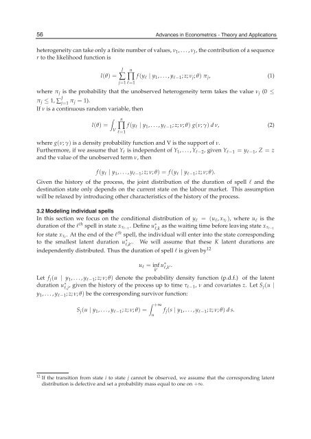
56 Advances in Econometrics - Theory and Applications10 Will-be-set-by-IN-TECHheterogeneity can take only a finite number of values, ν 1 ,...,ν J , the contribution of a sequencer to the likelihood function isl(θ) =J n∑ ∏ f (y l | y 1 ,...,y l−1 ; z; ν j ; θ) π j , (1)j=1 l=1where π j is the probability that the unobserved heterogeneity term takes the value ν j (0 ≤π j ≤ 1, ∑ J j=1 π j = 1).If ν is a continuous random variable, then∫l(θ) =n∏ f (y l | y 1 ,...,y l−1 ; z; ν; θ) g(ν; γ) d ν, (2)Vl=1where g(ν; γ) is a density probability function and V is the support of ν.Furthermore, if we assume that Y l is independent of Y 1 ,...,Y l−2 , given Y l−1 = y l−1 , Z = zand the value of the unobserved term ν, thenf (y l | y 1 ,...,y l−1 ; z; ν; θ) = f (y l | y l−1 ; z; ν; θ).Given the history of the process, the joint distribution of the duration of spell l and thedestination state only depends on the current state on the labour market. This assumptionwill be relaxed by introducing other characteristics of the history of the process.3.2 Modeling individual spellsIn this section we focus on the conditional distribution of y l= (u l , x τl ), where u l is theduration of the l th spell in state x τl−1 . Define u ∗ l,k as the waiting time before leaving state x τ l−1for state x τl . At the end of the l th spell, the individual will enter into the state correspondingto the smallest latent duration u ∗ l,k ′ . We will assume that these K latent durations areindependently distributed. Thus the duration of spell l is given by 12u l = infk ′ u ∗ l,k ′.Let f j (u | y 1 ,...,y l−1 ; z; ν; θ) denote the probability density function (p.d.f.) of the latentduration u ∗ l,j , given the history of the process up to time τ l−1, ν and covariates z. Let S j (u |y 1 ,...,y l−1 ; z; ν; θ) be the corresponding survivor function:S j (u | y 1 ,...,y l−1 ; z; ν; θ) =∫ +∞f j (s | y 1 ,...,y l−1 ; z; ν; θ) ds.u12 If the transition from state i to state j cannot be observed, we assume that the corresponding latentdistribution is defective and set a probability mass equal to one on +∞.