The Limits of Mathematics and NP Estimation in ... - Chichilnisky
The Limits of Mathematics and NP Estimation in ... - Chichilnisky
The Limits of Mathematics and NP Estimation in ... - Chichilnisky
- No tags were found...

Create successful ePaper yourself
Turn your PDF publications into a flip-book with our unique Google optimized e-Paper software.
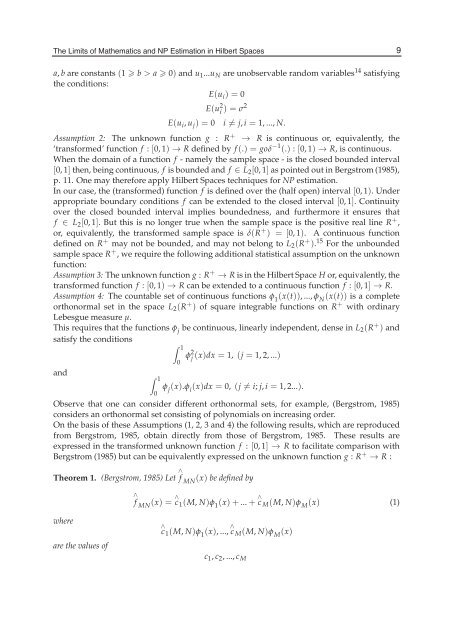
<strong>The</strong> <strong>Limits</strong> <strong>of</strong> <strong>Mathematics</strong><strong>and</strong> <strong>NP</strong> <strong>Estimation</strong> <strong>in</strong> Hilbert Spaces 7<strong>The</strong> <strong>Limits</strong> <strong>of</strong> <strong>Mathematics</strong> <strong>and</strong> <strong>NP</strong> <strong>Estimation</strong> <strong>in</strong> Hilbert Spacesa, b are constants (1 b > a 0) <strong>and</strong> u 1 ...u N are unobservable r<strong>and</strong>om variables 14 satisfy<strong>in</strong>gthe conditions:E(u i )=0E(u 2 i )=σ2E(u i , u j )=0 i ̸= j, i = 1, ..., N.Assumption 2: <strong>The</strong> unknown function g : R + → R is cont<strong>in</strong>uous or, equivalently, the‘transformed’ function f : [0, 1) → R def<strong>in</strong>ed by f (.) =goδ −1 (.) : [0, 1) → R, is cont<strong>in</strong>uous.When the doma<strong>in</strong> <strong>of</strong> a function f - namely the sample space - is the closed bounded <strong>in</strong>terval[0, 1] then, be<strong>in</strong>g cont<strong>in</strong>uous, f is bounded <strong>and</strong> f ∈ L 2 [0, 1] as po<strong>in</strong>ted out <strong>in</strong> Bergstrom (1985),p. 11. One may therefore apply Hilbert Spaces techniques for <strong>NP</strong> estimation.In our case, the (transformed) function f is def<strong>in</strong>ed over the (half open) <strong>in</strong>terval [0, 1). Underappropriate boundary conditions f can be extended to the closed <strong>in</strong>terval [0, 1]. Cont<strong>in</strong>uityover the closed bounded <strong>in</strong>terval implies boundedness, <strong>and</strong> furthermore it ensures thatf ∈ L 2 [0, 1]. But this is no longer true when the sample space is the positive real l<strong>in</strong>e R + ,or, equivalently, the transformed sample space is δ(R + ) = [0, 1). A cont<strong>in</strong>uous functiondef<strong>in</strong>ed on R + may not be bounded, <strong>and</strong> may not belong to L 2 (R + ). 15 For the unboundedsample space R + , we require the follow<strong>in</strong>g additional statistical assumption on the unknownfunction:Assumption 3: <strong>The</strong> unknown function g : R + → R is <strong>in</strong> the Hilbert Space H or, equivalently, thetransformed function f : [0, 1) → R can be extended to a cont<strong>in</strong>uous function f : [0, 1] → R.Assumption 4: <strong>The</strong> countable set <strong>of</strong> cont<strong>in</strong>uous functions φ 1(x(t)), ..., φ N(x(t)) is a completeorthonormal set <strong>in</strong> the space L 2 (R + ) <strong>of</strong> square <strong>in</strong>tegrable functions on R + with ord<strong>in</strong>aryLebesgue measure μ.This requires that the functions φ j be cont<strong>in</strong>uous, l<strong>in</strong>early <strong>in</strong>dependent, dense <strong>in</strong> L 2 (R + ) <strong>and</strong>satisfy the conditions∫ 1φ 2 j (x)dx = 1, (j = 1, 2, ...)0<strong>and</strong> ∫ 1φ j (x).φ i (x)dx = 0, (j ̸= i; j, i = 1, 2...).0Observe that one can consider different orthonormal sets, for example, (Bergstrom, 1985)considers an orthonormal set consist<strong>in</strong>g <strong>of</strong> polynomials on <strong>in</strong>creas<strong>in</strong>g order.On the basis <strong>of</strong> these Assumptions (1, 2, 3 <strong>and</strong> 4) the follow<strong>in</strong>g results, which are reproducedfrom Bergstrom, 1985, obta<strong>in</strong> directly from those <strong>of</strong> Bergstrom, 1985. <strong>The</strong>se results areexpressed <strong>in</strong> the transformed unknown function f : [0, 1] → R to facilitate comparison withBergstrom (1985) but can be equivalently expressed on the unknown function g : R + → R :<strong>The</strong>orem 1. (Bergstrom, 1985) Let ∧ f MN(x) be def<strong>in</strong>ed bywhereare the values <strong>of</strong>∧f MN (x) = ∧ c 1 (M, N)φ 1 (x)+... + ∧ c M (M, N)φ M (x) (1)∧c1 (M, N)φ 1 (x), ..., ∧ c M (M, N)φ M(x)c 1 , c 2 , ..., c M9