- Page 2 and 3:
APPLIEDDIFFERENTIALGEOMETRYA Modern
- Page 4 and 5:
APPLIEDDIFFERENTIALGEOMETRYA Modern
- Page 6 and 7:
Dedicated to:Nitya, Atma and Kali
- Page 8 and 9:
PrefaceApplied Differential Geometr
- Page 10 and 11:
ixAcknowledgmentsThe authors wish t
- Page 12 and 13:
Glossary of Frequently Used Symbols
- Page 14 and 15:
Glossary of Frequently Used Symbols
- Page 16 and 17:
Glossary of Frequently Used Symbols
- Page 18 and 19:
ContentsPrefaceGlossary of Frequent
- Page 20 and 21:
Contentsxix2.1.5.2 Forces Acting on
- Page 22 and 23:
Contentsxxi3.6.3.4 Stokes Theorem a
- Page 24 and 25:
Contentsxxiii3.10.3.1 Basis of Lagr
- Page 26 and 27:
Contentsxxv3.17 Applied Unorthodox
- Page 28 and 29:
Contentsxxvii4.9.8.2 Geometrodynami
- Page 30 and 31:
Contentsxxix4.14.7.5 Monopole Conde
- Page 32 and 33:
Contentsxxxi5.12.3 Hawking-Penrose
- Page 34 and 35:
Contentsxxxiii6.5.2.4 Dimensional R
- Page 36 and 37:
Chapter 1IntroductionIn this introd
- Page 38 and 39:
Introduction 3Fig. 1.1 The four cha
- Page 40 and 41:
Introduction 5• Riemannian manifo
- Page 42 and 43:
Introduction 7charts.The atlas cont
- Page 44 and 45:
Introduction 9every point has a nei
- Page 46 and 47:
Introduction 11of curves include ci
- Page 48 and 49:
Introduction 13the variables define
- Page 50 and 51:
Introduction 15U i denotes one of t
- Page 52 and 53:
Introduction 17which varies smoothl
- Page 54 and 55:
Introduction 19interactions.1.1.5.2
- Page 56 and 57:
Introduction 21real number. This co
- Page 58 and 59:
Introduction 23Such a force is inde
- Page 60 and 61:
Introduction 25tons. In this formul
- Page 62 and 63:
Introduction 27vector-field are sol
- Page 64 and 65:
Introduction 29or simply connected)
- Page 66 and 67:
Introduction 311.1.8 Application: A
- Page 68 and 69:
Introduction 33theory itself existe
- Page 70 and 71:
Introduction 35mediate the forces.
- Page 72 and 73:
Introduction 37theory. 50 Fig. 1.3
- Page 74 and 75:
Introduction 39to describe a univer
- Page 76 and 77:
Introduction 41which have two disti
- Page 78 and 79:
Introduction 43first theory can be
- Page 80 and 81:
Introduction 45the Casimir effect,
- Page 82 and 83:
Introduction 47• External coordin
- Page 84 and 85:
Introduction 49a connection-base de
- Page 86 and 87:
Chapter 2Technical Preliminaries: T
- Page 88 and 89:
Technical Preliminaries: Tensors, A
- Page 90 and 91:
Technical Preliminaries: Tensors, A
- Page 92 and 93:
Technical Preliminaries: Tensors, A
- Page 94 and 95:
Technical Preliminaries: Tensors, A
- Page 96 and 97:
Technical Preliminaries: Tensors, A
- Page 98 and 99:
Technical Preliminaries: Tensors, A
- Page 100 and 101:
Technical Preliminaries: Tensors, A
- Page 102 and 103:
Technical Preliminaries: Tensors, A
- Page 104 and 105:
Technical Preliminaries: Tensors, A
- Page 106 and 107:
Technical Preliminaries: Tensors, A
- Page 108 and 109:
Technical Preliminaries: Tensors, A
- Page 110 and 111:
Technical Preliminaries: Tensors, A
- Page 112 and 113:
Technical Preliminaries: Tensors, A
- Page 114 and 115:
Technical Preliminaries: Tensors, A
- Page 116 and 117:
Technical Preliminaries: Tensors, A
- Page 118 and 119:
Technical Preliminaries: Tensors, A
- Page 120 and 121:
Technical Preliminaries: Tensors, A
- Page 122 and 123:
Technical Preliminaries: Tensors, A
- Page 124 and 125:
Technical Preliminaries: Tensors, A
- Page 126 and 127:
Technical Preliminaries: Tensors, A
- Page 128 and 129:
Technical Preliminaries: Tensors, A
- Page 130 and 131:
Technical Preliminaries: Tensors, A
- Page 132 and 133:
Technical Preliminaries: Tensors, A
- Page 134 and 135:
Technical Preliminaries: Tensors, A
- Page 136 and 137:
Technical Preliminaries: Tensors, A
- Page 138 and 139:
Technical Preliminaries: Tensors, A
- Page 140 and 141:
Technical Preliminaries: Tensors, A
- Page 142 and 143:
Technical Preliminaries: Tensors, A
- Page 144 and 145:
Technical Preliminaries: Tensors, A
- Page 146 and 147:
Technical Preliminaries: Tensors, A
- Page 148 and 149:
Technical Preliminaries: Tensors, A
- Page 150 and 151:
Technical Preliminaries: Tensors, A
- Page 152 and 153:
Technical Preliminaries: Tensors, A
- Page 154 and 155:
Technical Preliminaries: Tensors, A
- Page 156 and 157:
Technical Preliminaries: Tensors, A
- Page 158 and 159:
Technical Preliminaries: Tensors, A
- Page 160 and 161:
Technical Preliminaries: Tensors, A
- Page 162 and 163:
Technical Preliminaries: Tensors, A
- Page 164 and 165:
Technical Preliminaries: Tensors, A
- Page 166 and 167:
Technical Preliminaries: Tensors, A
- Page 168 and 169:
Technical Preliminaries: Tensors, A
- Page 170 and 171:
Technical Preliminaries: Tensors, A
- Page 172 and 173:
Chapter 3Applied Manifold Geometry3
- Page 174 and 175:
Applied Manifold Geometry 139where
- Page 176 and 177:
Applied Manifold Geometry 141In loc
- Page 178 and 179:
Applied Manifold Geometry 143on the
- Page 180 and 181:
Applied Manifold Geometry 145exist
- Page 182 and 183:
Applied Manifold Geometry 147then E
- Page 184 and 185:
Applied Manifold Geometry 1490D man
- Page 186 and 187:
Applied Manifold Geometry 151Fig. 3
- Page 188 and 189:
Applied Manifold Geometry 153the fo
- Page 190 and 191:
Applied Manifold Geometry 155contin
- Page 192 and 193:
Applied Manifold Geometry 157In oth
- Page 194 and 195:
Applied Manifold Geometry 159scalar
- Page 196 and 197:
Applied Manifold Geometry 161where
- Page 198 and 199:
Applied Manifold Geometry 1633.6 Te
- Page 200 and 201:
Applied Manifold Geometry 165Let ϕ
- Page 202 and 203:
Applied Manifold Geometry 1673.6.1.
- Page 204 and 205:
Applied Manifold Geometry 169or, if
- Page 206 and 207:
Applied Manifold Geometry 171If X i
- Page 208 and 209:
Applied Manifold Geometry 173along
- Page 210 and 211:
Applied Manifold Geometry 175is dua
- Page 212 and 213:
Applied Manifold Geometry 177where
- Page 214 and 215:
Applied Manifold Geometry 179(1) α
- Page 216 and 217:
Applied Manifold Geometry 181diagra
- Page 218 and 219:
Applied Manifold Geometry 183Clearl
- Page 220 and 221:
Applied Manifold Geometry 1853.6.3.
- Page 222 and 223:
Applied Manifold Geometry 187duces,
- Page 224 and 225:
Applied Manifold Geometry 189This i
- Page 226 and 227:
Applied Manifold Geometry 191Hodge
- Page 228 and 229:
Applied Manifold Geometry 193The in
- Page 230 and 231:
Applied Manifold Geometry 195since
- Page 232 and 233:
Applied Manifold Geometry 197If a l
- Page 234 and 235:
Applied Manifold Geometry 199asGive
- Page 236 and 237:
Applied Manifold Geometry 201The co
- Page 238 and 239:
Applied Manifold Geometry 203at the
- Page 240 and 241:
Applied Manifold Geometry 205For ex
- Page 242 and 243:
Applied Manifold Geometry 207axis,
- Page 244 and 245:
Applied Manifold Geometry 209For ex
- Page 246 and 247:
Applied Manifold Geometry 211The sp
- Page 248 and 249:
Applied Manifold Geometry 213corres
- Page 250 and 251:
Applied Manifold Geometry 215corres
- Page 252 and 253:
Applied Manifold Geometry 217Specia
- Page 254 and 255:
Applied Manifold Geometry 219the co
- Page 256 and 257:
Applied Manifold Geometry 221moment
- Page 258 and 259:
Applied Manifold Geometry 223produc
- Page 260 and 261:
Applied Manifold Geometry 225has a
- Page 262 and 263:
Applied Manifold Geometry 2273.8.5
- Page 264 and 265:
Applied Manifold Geometry 229in whi
- Page 266 and 267:
Applied Manifold Geometry 231with
- Page 268 and 269:
Applied Manifold Geometry 233itly:(
- Page 270 and 271:
Applied Manifold Geometry 235play t
- Page 272 and 273:
Applied Manifold Geometry 237Some r
- Page 274 and 275:
Applied Manifold Geometry 239Basic
- Page 276 and 277:
Applied Manifold Geometry 241orthog
- Page 278 and 279:
Applied Manifold Geometry 243is adm
- Page 280 and 281:
Applied Manifold Geometry 245Root S
- Page 282 and 283:
Applied Manifold Geometry 247groups
- Page 284 and 285:
Applied Manifold Geometry 2493.9.1.
- Page 286 and 287:
Applied Manifold Geometry 251second
- Page 288 and 289:
Applied Manifold Geometry 253where
- Page 290 and 291:
Applied Manifold Geometry 255be a v
- Page 292 and 293:
Applied Manifold Geometry 257Now, a
- Page 294 and 295:
Applied Manifold Geometry 259This i
- Page 296 and 297:
Applied Manifold Geometry 2613.9.4
- Page 298 and 299:
Applied Manifold Geometry 263other
- Page 300 and 301:
Applied Manifold Geometry 265where
- Page 302 and 303:
Applied Manifold Geometry 267result
- Page 304 and 305:
Applied Manifold Geometry 269where
- Page 306 and 307:
Applied Manifold Geometry 2713.10 R
- Page 308 and 309:
Applied Manifold Geometry 273More p
- Page 310 and 311:
Applied Manifold Geometry 275Y (t 0
- Page 312 and 313:
Applied Manifold Geometry 277which
- Page 314 and 315:
Applied Manifold Geometry 279for an
- Page 316 and 317:
Applied Manifold Geometry 281where
- Page 318 and 319:
Applied Manifold Geometry 283Thus w
- Page 320 and 321:
Applied Manifold Geometry 2853.10.2
- Page 322 and 323:
Applied Manifold Geometry 287evolut
- Page 324 and 325:
Applied Manifold Geometry 2893.10.3
- Page 326 and 327:
Applied Manifold Geometry 2913.10.3
- Page 328 and 329:
Applied Manifold Geometry 293‘ren
- Page 330 and 331:
Applied Manifold Geometry 295mute;
- Page 332 and 333:
Applied Manifold Geometry 297Rather
- Page 334 and 335:
Applied Manifold Geometry 299of the
- Page 336 and 337:
Applied Manifold Geometry 301clidea
- Page 338 and 339:
Applied Manifold Geometry 303Second
- Page 340 and 341:
Applied Manifold Geometry 305i.e.,
- Page 342 and 343:
Applied Manifold Geometry 307invari
- Page 344 and 345:
Applied Manifold Geometry 309The Ba
- Page 346 and 347:
Applied Manifold Geometry 311Let us
- Page 348 and 349:
Applied Manifold Geometry 313all cu
- Page 350 and 351:
Applied Manifold Geometry 315ders.
- Page 352 and 353:
Applied Manifold Geometry 317this c
- Page 354 and 355:
Applied Manifold Geometry 319In par
- Page 356 and 357:
Applied Manifold Geometry 321As I p
- Page 358 and 359:
Applied Manifold Geometry 323the fo
- Page 360 and 361:
Applied Manifold Geometry 325per (1
- Page 362 and 363:
Applied Manifold Geometry 327Genera
- Page 364 and 365:
Applied Manifold Geometry 329The ma
- Page 366 and 367:
Applied Manifold Geometry 331pretat
- Page 368 and 369:
Applied Manifold Geometry 333byMDL
- Page 370 and 371:
Applied Manifold Geometry 3353.12 S
- Page 372 and 373:
Applied Manifold Geometry 337H 2 (M
- Page 374 and 375:
Applied Manifold Geometry 339bracke
- Page 376 and 377:
Applied Manifold Geometry 341Any so
- Page 378 and 379:
Applied Manifold Geometry 343All on
- Page 380 and 381:
Applied Manifold Geometry 345The ac
- Page 382 and 383:
Applied Manifold Geometry 347linear
- Page 384 and 385:
Applied Manifold Geometry 349such t
- Page 386 and 387:
Applied Manifold Geometry 351Let γ
- Page 388 and 389:
Applied Manifold Geometry 353This i
- Page 390 and 391:
Applied Manifold Geometry 355chart
- Page 392 and 393:
Applied Manifold Geometry 357phase-
- Page 394 and 395:
Applied Manifold Geometry 359( ) 0
- Page 396 and 397:
Applied Manifold Geometry 361hetero
- Page 398 and 399:
Applied Manifold Geometry 363thus c
- Page 400 and 401:
Applied Manifold Geometry 365Action
- Page 402 and 403:
Applied Manifold Geometry 367and we
- Page 404 and 405:
Applied Manifold Geometry 369action
- Page 406 and 407:
Applied Manifold Geometry 371and we
- Page 408 and 409:
Applied Manifold Geometry 373by (J(
- Page 410 and 411:
Applied Manifold Geometry 375fields
- Page 412 and 413:
Applied Manifold Geometry 377Let Tx
- Page 414 and 415:
Applied Manifold Geometry 379where
- Page 416 and 417:
Applied Manifold Geometry 381The ve
- Page 418 and 419:
Applied Manifold Geometry 383and gi
- Page 420 and 421:
Applied Manifold Geometry 385The co
- Page 422 and 423:
Applied Manifold Geometry 387tor Ca
- Page 424 and 425:
Applied Manifold Geometry 389where
- Page 426 and 427:
Applied Manifold Geometry 3912 −
- Page 428 and 429:
Applied Manifold Geometry 393comple
- Page 430 and 431:
Applied Manifold Geometry 395F[C]
- Page 432 and 433:
Applied Manifold Geometry 397become
- Page 434 and 435:
Applied Manifold Geometry 399of fuz
- Page 436 and 437:
Applied Manifold Geometry 401In our
- Page 438 and 439:
Applied Manifold Geometry 403Biodyn
- Page 440 and 441:
Applied Manifold Geometry 405for T
- Page 442 and 443:
Applied Manifold Geometry 407A vari
- Page 444 and 445:
Applied Manifold Geometry 409such t
- Page 446 and 447:
Applied Manifold Geometry 411of neg
- Page 448 and 449:
Applied Manifold Geometry 413where
- Page 450 and 451:
Applied Manifold Geometry 415Follow
- Page 452 and 453:
Applied Manifold Geometry 417and J
- Page 454 and 455:
Applied Manifold Geometry 419This t
- Page 456 and 457:
Applied Manifold Geometry 421above,
- Page 458 and 459:
Applied Manifold Geometry 423As a L
- Page 460 and 461:
Applied Manifold Geometry 425Theore
- Page 462 and 463:
Applied Manifold Geometry 427real v
- Page 464 and 465:
Applied Manifold Geometry 429indepe
- Page 466 and 467:
Applied Manifold Geometry 431In ter
- Page 468 and 469:
Applied Manifold Geometry 433M, we
- Page 470 and 471:
Applied Manifold Geometry 435The cu
- Page 472 and 473:
Applied Manifold Geometry 437(iv) (
- Page 474 and 475:
Applied Manifold Geometry 439where
- Page 476 and 477:
. ..Applied Manifold Geometry 441in
- Page 478 and 479:
Applied Manifold Geometry 443⌋ is
- Page 480 and 481:
Applied Manifold Geometry 445Now, a
- Page 482 and 483:
Applied Manifold Geometry 447symmet
- Page 484 and 485:
Applied Manifold Geometry 449study
- Page 486 and 487:
Applied Manifold Geometry 451togeth
- Page 488 and 489:
Applied Manifold Geometry 453result
- Page 490 and 491:
Applied Manifold Geometry 455will b
- Page 492 and 493:
Applied Manifold Geometry 457g 11 =
- Page 494 and 495:
Applied Manifold Geometry 459is def
- Page 496 and 497:
Applied Manifold Geometry 461ordere
- Page 498 and 499:
Applied Manifold Geometry 463Now, r
- Page 500 and 501:
Applied Manifold Geometry 465Simila
- Page 502 and 503:
Applied Manifold Geometry 467which
- Page 504 and 505:
Applied Manifold Geometry 469From t
- Page 506 and 507:
Applied Manifold Geometry 471where
- Page 508 and 509:
Applied Manifold Geometry 4733.17.2
- Page 510 and 511:
Applied Manifold Geometry 475On the
- Page 512 and 513:
Applied Manifold Geometry 477ing di
- Page 514 and 515:
Applied Manifold Geometry 479Note t
- Page 516 and 517:
Applied Manifold Geometry 481Then w
- Page 518 and 519:
Applied Manifold Geometry 483consis
- Page 520 and 521:
Chapter 4Applied Bundle Geometry4.1
- Page 522 and 523:
Applied Bundle Geometry 487is calle
- Page 524 and 525:
Applied Bundle Geometry 489V and an
- Page 526 and 527:
Applied Bundle Geometry 4914.3 Vect
- Page 528 and 529:
Applied Bundle Geometry 493dimensio
- Page 530 and 531:
Applied Bundle Geometry 495orthogon
- Page 532 and 533:
Applied Bundle Geometry 497t, is a
- Page 534 and 535:
Applied Bundle Geometry 499Let T Y
- Page 536 and 537:
Applied Bundle Geometry 501In other
- Page 538 and 539:
Applied Bundle Geometry 503we shall
- Page 540 and 541:
Applied Bundle Geometry 505Pendulum
- Page 542 and 543:
Applied Bundle Geometry 507Using L
- Page 544 and 545:
Applied Bundle Geometry 509the isom
- Page 546 and 547:
Applied Bundle Geometry 511theory f
- Page 548 and 549:
Applied Bundle Geometry 513of the c
- Page 550 and 551:
Applied Bundle Geometry 515where Ω
- Page 552 and 553:
Applied Bundle Geometry 517nals, th
- Page 554 and 555:
Applied Bundle Geometry 519(1985)])
- Page 556 and 557:
Applied Bundle Geometry 521finite-d
- Page 558 and 559:
Applied Bundle Geometry 523and thes
- Page 560 and 561:
Applied Bundle Geometry 525Now, let
- Page 562 and 563:
Applied Bundle Geometry 527gravity
- Page 564 and 565:
Applied Bundle Geometry 529a Dp−b
- Page 566 and 567:
Applied Bundle Geometry 531A princi
- Page 568 and 569:
Applied Bundle Geometry 533is the r
- Page 570 and 571:
Applied Bundle Geometry 535Now, let
- Page 572 and 573:
Applied Bundle Geometry 537By cycli
- Page 574 and 575:
Applied Bundle Geometry 5394.9.2 Fe
- Page 576 and 577: Applied Bundle Geometry 541This lin
- Page 578 and 579: Applied Bundle Geometry 543(1) L g
- Page 580 and 581: Applied Bundle Geometry 545and ω 0
- Page 582 and 583: Applied Bundle Geometry 547isfiesω
- Page 584 and 585: Applied Bundle Geometry 549of the c
- Page 586 and 587: Applied Bundle Geometry 551Controll
- Page 588 and 589: Applied Bundle Geometry 553Foliatio
- Page 590 and 591: Applied Bundle Geometry 555ψ : (x,
- Page 592 and 593: Applied Bundle Geometry 557from res
- Page 594 and 595: Applied Bundle Geometry 559Motion a
- Page 596 and 597: Applied Bundle Geometry 561where Z
- Page 598 and 599: Applied Bundle Geometry 563Systems
- Page 600 and 601: Applied Bundle Geometry 5653. Recal
- Page 602 and 603: Applied Bundle Geometry 567Therefor
- Page 604 and 605: Applied Bundle Geometry 569smooth m
- Page 606 and 607: Applied Bundle Geometry 571state va
- Page 608 and 609: Applied Bundle Geometry 573The geom
- Page 610 and 611: Applied Bundle Geometry 575Y ∋ y
- Page 612 and 613: Applied Bundle Geometry 577autonomo
- Page 614 and 615: Applied Bundle Geometry 579(see 3.1
- Page 616 and 617: Applied Bundle Geometry 581and init
- Page 618 and 619: Applied Bundle Geometry 583potentia
- Page 620 and 621: Applied Bundle Geometry 585effector
- Page 622 and 623: Applied Bundle Geometry 587Fig. 4.9
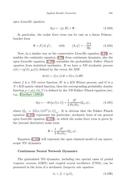
- Page 624 and 625: Applied Bundle Geometry 589physical
- Page 628 and 629: Applied Bundle Geometry 593et al. (
- Page 630 and 631: Applied Bundle Geometry 595(2) Acti
- Page 632 and 633: Applied Bundle Geometry 597˙Φ ≤
- Page 634 and 635: Applied Bundle Geometry 599number o
- Page 636 and 637: Applied Bundle Geometry 601where Ψ
- Page 638 and 639: Applied Bundle Geometry 603ing to c
- Page 640 and 641: Applied Bundle Geometry 605where [
- Page 642 and 643: Applied Bundle Geometry 607interval
- Page 644 and 645: Applied Bundle Geometry 609The foll
- Page 646 and 647: Applied Bundle Geometry 611In parti
- Page 648 and 649: Applied Bundle Geometry 613The pull
- Page 650 and 651: Applied Bundle Geometry 615(2) δ
- Page 652 and 653: Applied Bundle Geometry 617of unita
- Page 654 and 655: Applied Bundle Geometry 619system o
- Page 656 and 657: Applied Bundle Geometry 621of H pre
- Page 658 and 659: Applied Bundle Geometry 623It follo
- Page 660 and 661: Applied Bundle Geometry 625a produc
- Page 662 and 663: Applied Bundle Geometry 627B Ham(M)
- Page 664 and 665: Applied Bundle Geometry 629b.Let us
- Page 666 and 667: Applied Bundle Geometry 631If P is
- Page 668 and 669: Applied Bundle Geometry 633question
- Page 670 and 671: Applied Bundle Geometry 635spheres
- Page 672 and 673: Applied Bundle Geometry 637be thoug
- Page 674 and 675: Applied Bundle Geometry 639of the b
- Page 676 and 677:
Applied Bundle Geometry 641in C 1 (
- Page 678 and 679:
Applied Bundle Geometry 643from a t
- Page 680 and 681:
Applied Bundle Geometry 645Now let
- Page 682 and 683:
Applied Bundle Geometry 647for t <
- Page 684 and 685:
Applied Bundle Geometry 649is a Ham
- Page 686 and 687:
Applied Bundle Geometry 651The foll
- Page 688 and 689:
Applied Bundle Geometry 653is the u
- Page 690 and 691:
Applied Bundle Geometry 655every no
- Page 692 and 693:
Applied Bundle Geometry 657P × P w
- Page 694 and 695:
Applied Bundle Geometry 659that the
- Page 696 and 697:
Applied Bundle Geometry 661extend t
- Page 698 and 699:
Applied Bundle Geometry 663identity
- Page 700 and 701:
Applied Bundle Geometry 665The mapw
- Page 702 and 703:
Applied Bundle Geometry 667It is a
- Page 704 and 705:
Applied Bundle Geometry 669I Q is i
- Page 706 and 707:
Applied Bundle Geometry 671whereC i
- Page 708 and 709:
Applied Bundle Geometry 673form Q.
- Page 710 and 711:
Applied Bundle Geometry 675τ( exp(
- Page 712 and 713:
Applied Bundle Geometry 6774.13.2.2
- Page 714 and 715:
Applied Bundle Geometry 679Therefor
- Page 716 and 717:
Applied Bundle Geometry 6814.13.2.3
- Page 718 and 719:
Applied Bundle Geometry 683⎛⎞co
- Page 720 and 721:
Applied Bundle Geometry 685Usually,
- Page 722 and 723:
Applied Bundle Geometry 687on the s
- Page 724 and 725:
Applied Bundle Geometry 6894.13.2.5
- Page 726 and 727:
Applied Bundle Geometry 6914.13.3 P
- Page 728 and 729:
Applied Bundle Geometry 693Since T
- Page 730 and 731:
Applied Bundle Geometry 695On the o
- Page 732 and 733:
Applied Bundle Geometry 697may writ
- Page 734 and 735:
Applied Bundle Geometry 699determin
- Page 736 and 737:
Applied Bundle Geometry 701section,
- Page 738 and 739:
Applied Bundle Geometry 703for deri
- Page 740 and 741:
Applied Bundle Geometry 705dictions
- Page 742 and 743:
Applied Bundle Geometry 707too sing
- Page 744 and 745:
Applied Bundle Geometry 709In (4.18
- Page 746 and 747:
Applied Bundle Geometry 7114.13.4.4
- Page 748 and 749:
Applied Bundle Geometry 713sis repr
- Page 750 and 751:
Applied Bundle Geometry 7154.13.4.6
- Page 752 and 753:
Applied Bundle Geometry 717a (linea
- Page 754 and 755:
Applied Bundle Geometry 719past few
- Page 756 and 757:
Applied Bundle Geometry 721global q
- Page 758 and 759:
Applied Bundle Geometry 7239. It ha
- Page 760 and 761:
Applied Bundle Geometry 725needs to
- Page 762 and 763:
Applied Bundle Geometry 727pear at
- Page 764 and 765:
Applied Bundle Geometry 729X, F A i
- Page 766 and 767:
Applied Bundle Geometry 731ifolds,
- Page 768 and 769:
Applied Bundle Geometry 733and not
- Page 770 and 771:
Applied Bundle Geometry 735under U(
- Page 772 and 773:
Applied Bundle Geometry 737N = 2 br
- Page 774 and 775:
Applied Bundle Geometry 739thusa
- Page 776 and 777:
Applied Bundle Geometry 741antisymm
- Page 778 and 779:
Applied Bundle Geometry 743see this
- Page 780 and 781:
Applied Bundle Geometry 745Coupling
- Page 782 and 783:
Applied Bundle Geometry 747acts as
- Page 784 and 785:
Applied Bundle Geometry 749good coo
- Page 786 and 787:
Applied Bundle Geometry 751Φ. Brea
- Page 788 and 789:
Applied Bundle Geometry 753equating
- Page 790 and 791:
Applied Bundle Geometry 755differen
- Page 792 and 793:
Applied Bundle Geometry 7574.14.10
- Page 794 and 795:
Applied Bundle Geometry 759deformed
- Page 796 and 797:
Applied Bundle Geometry 761phenomen
- Page 798 and 799:
Applied Bundle Geometry 763appears
- Page 800 and 801:
Applied Bundle Geometry 7654.14.10.
- Page 802 and 803:
Applied Bundle Geometry 767For J >
- Page 804 and 805:
Applied Bundle Geometry 769K 1/2
- Page 806 and 807:
Applied Bundle Geometry 771(i) The
- Page 808 and 809:
Applied Bundle Geometry 773by α =
- Page 810 and 811:
Applied Bundle Geometry 775(4.279)
- Page 812 and 813:
Applied Bundle Geometry 777Λ ⊗
- Page 814 and 815:
Applied Bundle Geometry 779coupling
- Page 816 and 817:
Applied Bundle Geometry 781where we
- Page 818 and 819:
Applied Bundle Geometry 783The posi
- Page 820 and 821:
Applied Bundle Geometry 785Although
- Page 822 and 823:
Applied Bundle Geometry 787Let us a
- Page 824 and 825:
Applied Bundle Geometry 789of the t
- Page 826 and 827:
Applied Bundle Geometry 791The Riem
- Page 828 and 829:
Applied Bundle Geometry 793To compl
- Page 830 and 831:
Applied Bundle Geometry 795Ω 1 :Ω
- Page 832 and 833:
Chapter 5Applied Jet GeometryModern
- Page 834 and 835:
Applied Jet Geometry 799x, with coe
- Page 836 and 837:
Applied Jet Geometry 801s i (x), as
- Page 838 and 839:
Applied Jet Geometry 803It is conve
- Page 840 and 841:
Applied Jet Geometry 805has the 1
- Page 842 and 843:
Applied Jet Geometry 807which split
- Page 844 and 845:
Applied Jet Geometry 809gives the h
- Page 846 and 847:
Applied Jet Geometry 811Furthermore
- Page 848 and 849:
Applied Jet Geometry 813This is a c
- Page 850 and 851:
Applied Jet Geometry 815Due to this
- Page 852 and 853:
Applied Jet Geometry 817The affine
- Page 854 and 855:
Applied Jet Geometry 819In particul
- Page 856 and 857:
Applied Jet Geometry 821Building on
- Page 858 and 859:
Applied Jet Geometry 823on J ∞ (X
- Page 860 and 861:
Applied Jet Geometry 825its tangent
- Page 862 and 863:
Applied Jet Geometry 827Fig. 5.3 Hi
- Page 864 and 865:
Applied Jet Geometry 829It follows
- Page 866 and 867:
Applied Jet Geometry 831affine, whi
- Page 868 and 869:
Applied Jet Geometry 833where Γ i
- Page 870 and 871:
Applied Jet Geometry 8355.6.5 Jacob
- Page 872 and 873:
Applied Jet Geometry 837is also the
- Page 874 and 875:
Applied Jet Geometry 839A generic m
- Page 876 and 877:
Applied Jet Geometry 841where ϑ eH
- Page 878 and 879:
Applied Jet Geometry 843Since E L|
- Page 880 and 881:
Applied Jet Geometry 845Thus, every
- Page 882 and 883:
Applied Jet Geometry 847along u. Ev
- Page 884 and 885:
Applied Jet Geometry 849equations c
- Page 886 and 887:
Applied Jet Geometry 851A Hamiltoni
- Page 888 and 889:
Applied Jet Geometry 853Connections
- Page 890 and 891:
Applied Jet Geometry 855Lagrangian
- Page 892 and 893:
Applied Jet Geometry 857on V ∗ M.
- Page 894 and 895:
Applied Jet Geometry 859contain no
- Page 896 and 897:
Applied Jet Geometry 861(ii) For an
- Page 898 and 899:
Applied Jet Geometry 8635.6.16 Lyap
- Page 900 and 901:
Applied Jet Geometry 865for any t >
- Page 902 and 903:
Applied Jet Geometry 867vertical co
- Page 904 and 905:
Applied Jet Geometry 869difficulty,
- Page 906 and 907:
Applied Jet Geometry 871the energy
- Page 908 and 909:
Applied Jet Geometry 873by the tran
- Page 910 and 911:
Applied Jet Geometry 875The conditi
- Page 912 and 913:
Applied Jet Geometry 877Let Γ = (M
- Page 914 and 915:
Applied Jet Geometry 879geometrical
- Page 916 and 917:
Applied Jet Geometry 881Let (M, I)
- Page 918 and 919:
Applied Jet Geometry 883so referrin
- Page 920 and 921:
Applied Jet Geometry 885The Poincar
- Page 922 and 923:
Applied Jet Geometry 887where N n
- Page 924 and 925:
Applied Jet Geometry 889be a projec
- Page 926 and 927:
Applied Jet Geometry 891to differen
- Page 928 and 929:
Applied Jet Geometry 893for every c
- Page 930 and 931:
Applied Jet Geometry 895vector-fiel
- Page 932 and 933:
Applied Jet Geometry 897This is phr
- Page 934 and 935:
Applied Jet Geometry 899where a, b
- Page 936 and 937:
Applied Jet Geometry 901represent t
- Page 938 and 939:
Applied Jet Geometry 903̂L : J 1 (
- Page 940 and 941:
Applied Jet Geometry 905space J 1 (
- Page 942 and 943:
Applied Jet Geometry 907First of al
- Page 944 and 945:
Applied Jet Geometry 909Therefore,
- Page 946 and 947:
Applied Jet Geometry 911Recall that
- Page 948 and 949:
Applied Jet Geometry 9135.11 Applic
- Page 950 and 951:
Applied Jet Geometry 915the vector
- Page 952 and 953:
Applied Jet Geometry 9175.11.4 Gaug
- Page 954 and 955:
Applied Jet Geometry 9195.11.5 Lagr
- Page 956 and 957:
Applied Jet Geometry 921are represe
- Page 958 and 959:
Applied Jet Geometry 923which are t
- Page 960 and 961:
Applied Jet Geometry 925of this fun
- Page 962 and 963:
Applied Jet Geometry 927a principal
- Page 964 and 965:
Applied Jet Geometry 929Recall that
- Page 966 and 967:
Applied Jet Geometry 931Moreover, t
- Page 968 and 969:
Applied Jet Geometry 933other only
- Page 970 and 971:
Applied Jet Geometry 935In particul
- Page 972 and 973:
Applied Jet Geometry 937Note that,
- Page 974 and 975:
Applied Jet Geometry 939This equali
- Page 976 and 977:
Applied Jet Geometry 941Then, the s
- Page 978 and 979:
Applied Jet Geometry 943In the Lagr
- Page 980 and 981:
Applied Jet Geometry 945Let τ be a
- Page 982 and 983:
Applied Jet Geometry 947Using (5.42
- Page 984 and 985:
Applied Jet Geometry 949associated
- Page 986 and 987:
Applied Jet Geometry 951parts,F α
- Page 988 and 989:
Applied Jet Geometry 953of the Hilb
- Page 990 and 991:
Applied Jet Geometry 955For example
- Page 992 and 993:
Applied Jet Geometry 957the convent
- Page 994 and 995:
Applied Jet Geometry 959left ideal
- Page 996 and 997:
Applied Jet Geometry 961LX → Σ i
- Page 998 and 999:
Applied Jet Geometry 963Levi-Civita
- Page 1000 and 1001:
Applied Jet Geometry 965see this fr
- Page 1002 and 1003:
Applied Jet Geometry 967curves. And
- Page 1004 and 1005:
Applied Jet Geometry 969One sees th
- Page 1006 and 1007:
Applied Jet Geometry 971sums over a
- Page 1008 and 1009:
Applied Jet Geometry 973all this to
- Page 1010 and 1011:
Applied Jet Geometry 975universe ev
- Page 1012 and 1013:
Applied Jet Geometry 977on Σ. If M
- Page 1014 and 1015:
Applied Jet Geometry 979(1) Lorentz
- Page 1016 and 1017:
Applied Jet Geometry 981terpret thi
- Page 1018 and 1019:
Chapter 6Geometrical Path Integrals
- Page 1020 and 1021:
Geometrical Path Integrals and Thei
- Page 1022 and 1023:
Geometrical Path Integrals and Thei
- Page 1024 and 1025:
Geometrical Path Integrals and Thei
- Page 1026 and 1027:
Geometrical Path Integrals and Thei
- Page 1028 and 1029:
Geometrical Path Integrals and Thei
- Page 1030 and 1031:
Geometrical Path Integrals and Thei
- Page 1032 and 1033:
Geometrical Path Integrals and Thei
- Page 1034 and 1035:
Geometrical Path Integrals and Thei
- Page 1036 and 1037:
Geometrical Path Integrals and Thei
- Page 1038 and 1039:
Geometrical Path Integrals and Thei
- Page 1040 and 1041:
Geometrical Path Integrals and Thei
- Page 1042 and 1043:
Geometrical Path Integrals and Thei
- Page 1044 and 1045:
Geometrical Path Integrals and Thei
- Page 1046 and 1047:
Geometrical Path Integrals and Thei
- Page 1048 and 1049:
Geometrical Path Integrals and Thei
- Page 1050 and 1051:
Geometrical Path Integrals and Thei
- Page 1052 and 1053:
Geometrical Path Integrals and Thei
- Page 1054 and 1055:
Geometrical Path Integrals and Thei
- Page 1056 and 1057:
Geometrical Path Integrals and Thei
- Page 1058 and 1059:
Geometrical Path Integrals and Thei
- Page 1060 and 1061:
Geometrical Path Integrals and Thei
- Page 1062 and 1063:
Geometrical Path Integrals and Thei
- Page 1064 and 1065:
Geometrical Path Integrals and Thei
- Page 1066 and 1067:
Geometrical Path Integrals and Thei
- Page 1068 and 1069:
Geometrical Path Integrals and Thei
- Page 1070 and 1071:
Geometrical Path Integrals and Thei
- Page 1072 and 1073:
Geometrical Path Integrals and Thei
- Page 1074 and 1075:
Geometrical Path Integrals and Thei
- Page 1076 and 1077:
Geometrical Path Integrals and Thei
- Page 1078 and 1079:
Geometrical Path Integrals and Thei
- Page 1080 and 1081:
Geometrical Path Integrals and Thei
- Page 1082 and 1083:
Geometrical Path Integrals and Thei
- Page 1084 and 1085:
Geometrical Path Integrals and Thei
- Page 1086 and 1087:
Geometrical Path Integrals and Thei
- Page 1088 and 1089:
Geometrical Path Integrals and Thei
- Page 1090 and 1091:
Geometrical Path Integrals and Thei
- Page 1092 and 1093:
Geometrical Path Integrals and Thei
- Page 1094 and 1095:
Geometrical Path Integrals and Thei
- Page 1096 and 1097:
Geometrical Path Integrals and Thei
- Page 1098 and 1099:
Geometrical Path Integrals and Thei
- Page 1100 and 1101:
Geometrical Path Integrals and Thei
- Page 1102 and 1103:
Geometrical Path Integrals and Thei
- Page 1104 and 1105:
Geometrical Path Integrals and Thei
- Page 1106 and 1107:
Geometrical Path Integrals and Thei
- Page 1108 and 1109:
Geometrical Path Integrals and Thei
- Page 1110 and 1111:
Geometrical Path Integrals and Thei
- Page 1112 and 1113:
Geometrical Path Integrals and Thei
- Page 1114 and 1115:
Geometrical Path Integrals and Thei
- Page 1116 and 1117:
Geometrical Path Integrals and Thei
- Page 1118 and 1119:
Geometrical Path Integrals and Thei
- Page 1120 and 1121:
Geometrical Path Integrals and Thei
- Page 1122 and 1123:
Geometrical Path Integrals and Thei
- Page 1124 and 1125:
Geometrical Path Integrals and Thei
- Page 1126 and 1127:
Geometrical Path Integrals and Thei
- Page 1128 and 1129:
Geometrical Path Integrals and Thei
- Page 1130 and 1131:
Geometrical Path Integrals and Thei
- Page 1132 and 1133:
Geometrical Path Integrals and Thei
- Page 1134 and 1135:
Geometrical Path Integrals and Thei
- Page 1136 and 1137:
Geometrical Path Integrals and Thei
- Page 1138 and 1139:
Geometrical Path Integrals and Thei
- Page 1140 and 1141:
Geometrical Path Integrals and Thei
- Page 1142 and 1143:
Geometrical Path Integrals and Thei
- Page 1144 and 1145:
Geometrical Path Integrals and Thei
- Page 1146 and 1147:
Geometrical Path Integrals and Thei
- Page 1148 and 1149:
Geometrical Path Integrals and Thei
- Page 1150 and 1151:
Geometrical Path Integrals and Thei
- Page 1152 and 1153:
Geometrical Path Integrals and Thei
- Page 1154 and 1155:
Geometrical Path Integrals and Thei
- Page 1156 and 1157:
Geometrical Path Integrals and Thei
- Page 1158 and 1159:
Geometrical Path Integrals and Thei
- Page 1160 and 1161:
Geometrical Path Integrals and Thei
- Page 1162 and 1163:
Geometrical Path Integrals and Thei
- Page 1164 and 1165:
Geometrical Path Integrals and Thei
- Page 1166 and 1167:
Geometrical Path Integrals and Thei
- Page 1168 and 1169:
Geometrical Path Integrals and Thei
- Page 1170 and 1171:
Geometrical Path Integrals and Thei
- Page 1172 and 1173:
Geometrical Path Integrals and Thei
- Page 1174 and 1175:
Geometrical Path Integrals and Thei
- Page 1176 and 1177:
Geometrical Path Integrals and Thei
- Page 1178 and 1179:
Geometrical Path Integrals and Thei
- Page 1180 and 1181:
Geometrical Path Integrals and Thei
- Page 1182 and 1183:
Geometrical Path Integrals and Thei
- Page 1184 and 1185:
Geometrical Path Integrals and Thei
- Page 1186 and 1187:
Geometrical Path Integrals and Thei
- Page 1188 and 1189:
Geometrical Path Integrals and Thei
- Page 1190 and 1191:
Geometrical Path Integrals and Thei
- Page 1192 and 1193:
Geometrical Path Integrals and Thei
- Page 1194 and 1195:
Geometrical Path Integrals and Thei
- Page 1196 and 1197:
Geometrical Path Integrals and Thei
- Page 1198 and 1199:
Geometrical Path Integrals and Thei
- Page 1200 and 1201:
Geometrical Path Integrals and Thei
- Page 1202 and 1203:
Geometrical Path Integrals and Thei
- Page 1204 and 1205:
Geometrical Path Integrals and Thei
- Page 1206 and 1207:
Geometrical Path Integrals and Thei
- Page 1208 and 1209:
Geometrical Path Integrals and Thei
- Page 1210 and 1211:
Geometrical Path Integrals and Thei
- Page 1212 and 1213:
Geometrical Path Integrals and Thei
- Page 1214 and 1215:
Geometrical Path Integrals and Thei
- Page 1216 and 1217:
Geometrical Path Integrals and Thei
- Page 1218 and 1219:
Geometrical Path Integrals and Thei
- Page 1220 and 1221:
Geometrical Path Integrals and Thei
- Page 1222 and 1223:
Geometrical Path Integrals and Thei
- Page 1224 and 1225:
Geometrical Path Integrals and Thei
- Page 1226 and 1227:
Geometrical Path Integrals and Thei
- Page 1228 and 1229:
Geometrical Path Integrals and Thei
- Page 1230 and 1231:
Geometrical Path Integrals and Thei
- Page 1232 and 1233:
Geometrical Path Integrals and Thei
- Page 1234 and 1235:
Geometrical Path Integrals and Thei
- Page 1236 and 1237:
Geometrical Path Integrals and Thei
- Page 1238 and 1239:
Geometrical Path Integrals and Thei
- Page 1240 and 1241:
Geometrical Path Integrals and Thei
- Page 1242 and 1243:
Geometrical Path Integrals and Thei
- Page 1244 and 1245:
Geometrical Path Integrals and Thei
- Page 1246 and 1247:
Geometrical Path Integrals and Thei
- Page 1248 and 1249:
Geometrical Path Integrals and Thei
- Page 1250 and 1251:
Geometrical Path Integrals and Thei
- Page 1252 and 1253:
Geometrical Path Integrals and Thei
- Page 1254 and 1255:
Geometrical Path Integrals and Thei
- Page 1256 and 1257:
Geometrical Path Integrals and Thei
- Page 1258 and 1259:
Geometrical Path Integrals and Thei
- Page 1260 and 1261:
Geometrical Path Integrals and Thei
- Page 1262 and 1263:
Geometrical Path Integrals and Thei
- Page 1264 and 1265:
Geometrical Path Integrals and Thei
- Page 1266 and 1267:
Geometrical Path Integrals and Thei
- Page 1268 and 1269:
Geometrical Path Integrals and Thei
- Page 1270 and 1271:
Geometrical Path Integrals and Thei
- Page 1272 and 1273:
Geometrical Path Integrals and Thei
- Page 1274 and 1275:
Geometrical Path Integrals and Thei
- Page 1276 and 1277:
Geometrical Path Integrals and Thei
- Page 1278 and 1279:
Geometrical Path Integrals and Thei
- Page 1280 and 1281:
Geometrical Path Integrals and Thei
- Page 1282 and 1283:
Geometrical Path Integrals and Thei
- Page 1284 and 1285:
Geometrical Path Integrals and Thei
- Page 1286 and 1287:
Geometrical Path Integrals and Thei
- Page 1288 and 1289:
BibliographyAblowitz, M.J., Clarkso
- Page 1290 and 1291:
Bibliography 1255equations. Springe
- Page 1292 and 1293:
Bibliography 1257connections, Phys.
- Page 1294 and 1295:
Bibliography 1259JHEP 0003:007.Bran
- Page 1296 and 1297:
Bibliography 1261Clementi, C. Petti
- Page 1298 and 1299:
Bibliography 1263Domany, E., Van He
- Page 1300 and 1301:
Bibliography 1265geometrical signat
- Page 1302 and 1303:
Bibliography 1267Bergmann theory of
- Page 1304 and 1305:
Bibliography 1269to Complex Systems
- Page 1306 and 1307:
Bibliography 1271Action for String
- Page 1308 and 1309:
Bibliography 1273Ivancevic, V., Bea
- Page 1310 and 1311:
Bibliography 1275Krener, A. (1984).
- Page 1312 and 1313:
Bibliography 1277Li, M., Vitanyi, P
- Page 1314 and 1315:
Bibliography 1279Nature, 261(5560),
- Page 1316 and 1317:
Bibliography 1281Lambert and R. Gol
- Page 1318 and 1319:
Bibliography 1283dynamics of human
- Page 1320 and 1321:
Bibliography 1285Reshetikhin, N.Yu,
- Page 1322 and 1323:
Bibliography 1287Rev. E, 58, 6333-6
- Page 1324 and 1325:
Bibliography 1289Stasheff, J.D. (19
- Page 1326 and 1327:
Bibliography 1291matical Physics. S
- Page 1328 and 1329:
Bibliography 1293Witten, E. (1991).
- Page 1330 and 1331:
Index1−jet bundle, 8271−jet lif
- Page 1332 and 1333:
Index 1297Chan-Paton factor, 1238Ch
- Page 1334 and 1335:
Index 1299Dirac-Born-Infeld theory,
- Page 1336 and 1337:
Index 1301Gauss, 5Gauss map, 284Gau
- Page 1338 and 1339:
Index 1303isometric, 17isomorphic,
- Page 1340 and 1341:
Index 1305Maxwell Lagrangian, 34Max
- Page 1342 and 1343:
Index 1307probability manifold, 333
- Page 1344 and 1345:
Index 1309super-space, 1215supercov
- Page 1346:
Index 1311Yang-Mills theory, 39, 29