DOTcvpSB: a Matlab Toolbox for Dynamic Optimization in Systems ...

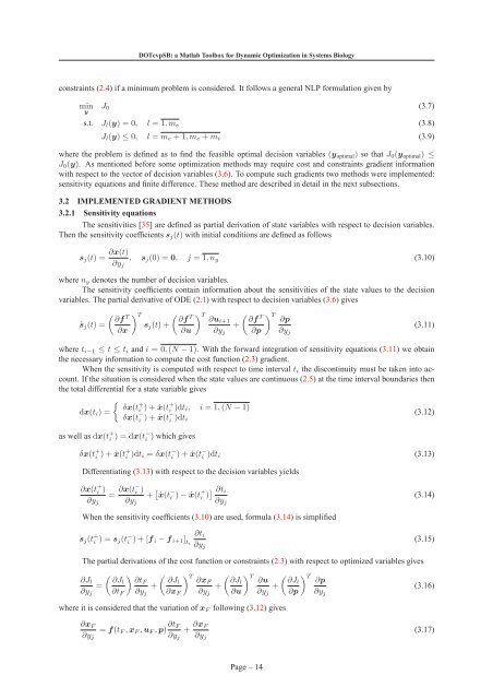
DOTcvpSB: a Matlab Toolbox for Dynamic Optimization in Systems Biologyconstraints (2.4) if a minimum problem is considered. It follows a general NLP formulation given byminyJ 0 (3.7)s.t. J l (y) = 0, l = 1,m e (3.8)J l (y) ≤ 0, l = m e +1,m e +m i (3.9)where the problem is defined as to find the feasible optimal decision variables (y optimal ) so that J 0 (y optimal ) ≤J 0 (y). As mentioned before some optimization methods may require cost and constraints gradient informationwith respect to the vector of decision variables (3.6). To compute such gradients two methods were implemented:sensitivity equations and finite difference. These method are described in detail in the next subsections.3.2 IMPLEMENTED GRADIENT METHODS3.2.1 Sensitivity equationsThe sensitivities [35] are defined as partial derivation of state variables with respect to decision variables.Then the sensitivity coefficients s j (t) with initial conditions are defined as followss j (t) = ∂x(t)∂y j, s j (0) = 0, j = 1,n y (3.10)where n y denotes the number of decision variables.The sensitivity coefficients contain information about the sensitivities of the state values to the decisionvariables. The partial derivative of ODE (2.1) with respect to decision variables (3.6) gives( ) ∂fT T∂fTṡ j (t) = s j (t)+(∂x ∂u) T ( )∂ui+1 ∂fT T∂p+(3.11)∂y j ∂p ∂y jwhere t i−1 ≤ t ≤ t i and i = 0,(N −1). With the forward integration of sensitivity equations (3.11) we obtainthe necessary information to compute the cost function (2.3) gradient.When the sensitivity is computed with respect to time interval t i the discontinuity must be taken into account.If the situation is considered when the state values are continuous (2.5) at the time interval boundaries thenthe total differential for a state variable givesdx(t i ) ={δx(t+i )+ẋ(t+ i )dt i, i = 1,(N −1)δx(t − i )+ẋ(t− i )dt i(3.12)as well as dx(t + i ) = dx(t− i ) which givesδx(t + i )+ẋ(t+ i )dt i = δx(t − i )+ẋ(t− i )dt i (3.13)Differentiating (3.13) with respect to the decision variables yields∂x(t + i ) = ∂x(t− i ) + [ ẋ(t − i∂y j ∂y )−ẋ(t+ i )] ∂t i(3.14)j ∂y jWhen the sensitivity coefficients (3.10) are used, formula (3.14) is simplifieds j (t + i ) = s j(t − i )+[f i −f i+1 ] ti∂t i∂y j(3.15)The partial derivations of the cost function or constraints (2.3) with respect to optimized variables gives( ) ( ) T∂J l ∂Jl ∂tF ∂Jl ∂x F= + +∂y j ∂t F ∂y j ∂x F ∂y j( ) T ∂Jl ∂u+∂u ∂y jwhere it is considered that the variation of x F following (3.12) gives( ) T ∂Jl ∂p(3.16)∂p ∂y j∂x F∂y j= f(t F ,x F ,u F ,p) ∂t F∂y j+ ∂x F∂y j(3.17)Page – 14