DOTcvpSB: a Matlab Toolbox for Dynamic Optimization in Systems ...

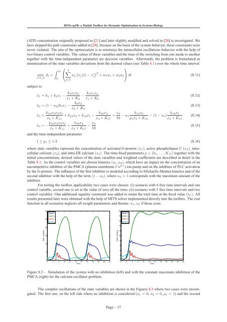
DOTcvpSB: a Matlab Toolbox for Dynamic Optimization in Systems Biology(ATP) concentration originally proposed in [21] and later slightly modified and solved in [28] is investigated. Wehave skipped the path constraints added in [28], because on the basis of the system behavior, these constraints werenever violated. The aim of the optimization is to minimize the intracellular oscillations behavior with the help oftwo binary control variables. The values of these variables and the time of the switching from one mode to anothertogether with the time-independent parameter are decision variables. Afterwards, the problem is formulated asminimization of the state variables deviations from the desired values (see Table 8.1) over the whole time intervalsubject to∫ tFmin J 0 =x,u i,p0⎛⎝4∑j=1⎞(w j xj (t)−x s ) 2j +w5 u 1 +w 6 u 2⎠dt (8.11)ẋ 1 = k 1 +k 2 x 1 − k 3x 1 x 2x 1 +K 4− k 5x 1 x 3x 1 +K 6(8.12)ẋ 2 = (1−u 2 )k 7 x 1 − k 8x 2x 2 +K 9(8.13)ẋ 3 = k 10x 2 x 3 x 4+k 12 x 2 +k 13 x 1 − k 16x 3+ x 4x 4 +K 11 x 3 +K 17 10 −u k 14 x 3 k 14 x 31 −(1−u 1 )p 1 x 3 +K 15 x 3 +K 15(8.14)ẋ 4 = − k 10x 2 x 3 x 4x 4 +K 11+ k 16x 3x 3 +K 17− x 410and the time-independent parameter(8.15)1 ≤ p 1 ≤ 1.3 (8.16)where state variables represent the concentration of activated G-protein (x 1 ), active phospholipase C (x 2 ), intracellularcalcium (x 3 ), and intra-ER calcium (x 4 ). The time-fixed parameters p = (k 1 ,...,K 17 ) together with theinitial concentrations, desired values of the state variables and weighted coefficients are described in detail in theTable 8.1. As the control variables are chosen binaries (u 1 ,u 2 ), which have an impact on the concentration of anuncompetitive inhibitor of the PMCA (plasma membrane Ca 2+ ) ion pump and on the inhibitor of PLC activationby the G-protein. The influence of the first inhibitor is modeled according to Michaelis-Menten kinetics and of thesecond inhibitor with the help of the term (1−u 2 ), where u 2 = 1 corresponds with the maximum amount of theinhibitor.For testing the toolbox applicability two cases were chosen: (i) scenario with 6 free time intervals and onecontrol variable, second one is set at the value of zero all the time; (ii) scenario with 5 free time intervals and twocontrol variables. One additional equality constraint was added to retain the total time at the fixed value (t F ). Allresults presented later were obtained with the help of MITS solver implemented directly into the toolbox. The costfunction in all scenarios neglects all weight parameters and therms: u 1 ,u 2 if those exist.3020x 1x 1x 218x 225x 316x 40 2 4 6 8 10 12 14 16 18 20 22x 3x 4State variables201510State variables1412108654200 2 4 6 8 10 12 14 16 18 20 22Time0TimeFigure 8.3 – Simulation of the system with no inhibition (left) and with the constant maximum inhibition of thePMCA (right) for the calcium oscillator problem.The complex oscillations of the state variables are shown in the Figures 8.3 where two cases were investigated.The first one, on the left side where no inhibition is considered (u 1 = 0, u 2 = 0, p 1 = 1) and the secondPage – 37