Laporan Akhir Projek Penyelidikan Jangka Pendek ... - ePrints@USM

More documents

Recommendations

Info

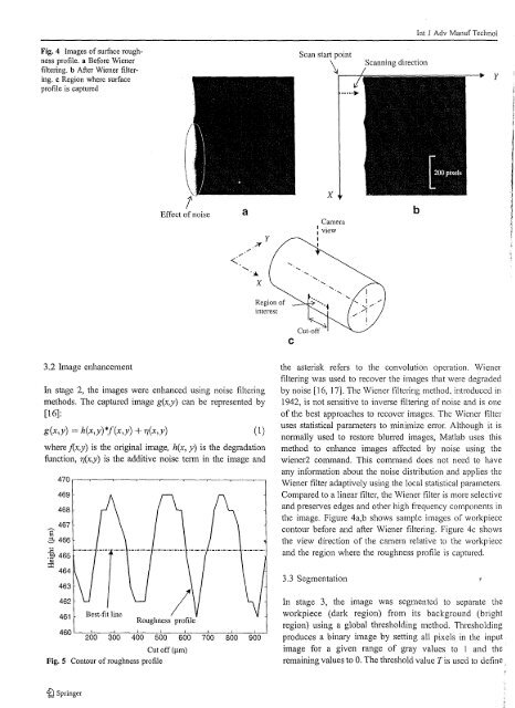
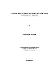
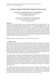
Int J Adv Manuf TechnolFig. 4 Images of surface roughnessprofile. a Before Wienerfiltering. b After Wiener filtering.c Region where surfaceprotile is capturedScan start point\Scanning directionyEffect of noise/.?fyxCameraI .I viewIIbRegion ofimeresl3.2 Image enhancementIn stage 2, the images were enhanced using noise filteringmethods. The captured image g(x,y) can be represented by[16]:g(x,y) = h(x,y)*f(x,y) + 7J(x,y) (1)where j(x,y) is the original image, hex, y) is the degradationfunction, 7J(x,y) is the additive noise term in the image and470 '--"'--~--"----~-~--"'-----'--r---o469468467Ẹ 3 466~Q 465~ 464463461Best-fit lineRoughness profile460 L.--::-'-=-~'-o---:~-::-::-::---=-'-::---=~-~--::-7-=--'200 300 400 500 600 700 800 900Cut off (I.tm)Fig. 5 Contour of roughness profilethe asterisk refers to the convolution operation. Wienerfiltering was used to recover the images that were degradedby noise [16, 17]. The Wiener filtering method, introduced in1942, is not sensitive to inverse filtering of noise and is oneof the best approaches to recover images. The Wiener filteruses statistical parameters to minimize error. Although it isnonnally used to restore blU11'ed images, Matlab uses thismethod to enhance images affected by noise using thewiener2 command. This command does not need to haveany infonnation about the noise distribution and applies theWiener filter adaptively using the local statistical parameters.Compared to a linear filter, the Wiener filter is more selectiveand preserves edges and other high frequency components inthe image. Figure 4a,b shows sample images of workpiececontour before and after Wiener filtering. Figure 4c showsthe view direction of the camera relative to the workpieceand the region where the roughness profile is captured.3.3 SegmentationIn stage 3, the image was segmented to separate theworkpiece (dark region) from its background (brightregion) using a global thresholding method. Thresholdingproduces a binary image by setting all pixels in the inputimage for a given range of gray values to 1 and theremaining values to O. The threshold value T is used to define.tQ Springer
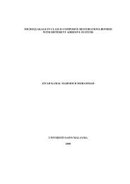
Int J Adv Manuf TechnolTable 4 Comparison between roughness determined using vision method and stylus methodIR"(s)-R"(vllCutting speed (m/min) Feed rate (mm/rev) R,,(v) ~m R,,(s) ~mR"(s)(xIOO%)Rq(v) ~m Rq(s) ~111!R./,) R.,(,·i!R.,(s)(xIOO%)16.3 0.2 1.81 1.75 3.4% 2.14 2.10 1.9%0.25 2.50 2.62 4.6% 2.87 3.03 5.3%0.3 3.25 3.23 0.6% 3.73 3.77 1.1%0.4 5.23 4.95 5.7% 6.28 6.04 4.0'Yo23.8 0.2 1.72 1.76 2.3% 2.00 2.18 8.3%0.25 2.96 2.69 10.0% 3.41 3.13 9.0'Yo0.3 3.38 3.49 3.2% 3.97 4.10 3.2%0.4 6.82 6.70 1.8% 8.02 7.78 3.1%39.6 0.2 1.74 1.76 1.1% 2.06 2.18 5.5%0.25 2.58 2.67 3.4% 3.06 3.23 5.3%0.3 2.61 2.64 1.1% 3.11 3.15 1.3%0.4 6.48 6.42 0.9% 7.66 7.63 0.4%K,(v) and Rq(v): Roughness determined using vision method.Rq(s) and R,is): Roughness measured using stylus method.the range of grayscale values that are set to 0 and 1. Twasdetermined automaticaily using the "graythresh" command inMatlab that uses the well-known Otsu's method [18]. Otsu'salgorithm uses the image histogram to detennine thethreshold value. The algorithm assumes that the imagehistogram is bimodal and detennines the optimum thresholdvalue that separates the two groups of pixels.3.4 Roughness measurementThe captured image shows the workpiece surface contourand the roughness value can be determined directly fromthe image without the need of a stylus method. In stage 4,the surface contour in the binarized image was detectedusing an algorithm written in Matlab. Each image is read asa matrix ofX and Y (row by column). Since in the binarizedimages, white areas have an intensity value of 1 and black7r--,---;:=====:::::;-r---~--~6 I X Stylus method I• Vision method5areas have an intensity value of 0, the surface profile of theworkpiece is detected when the intensity value changesfrom I to O. The algorithm starts scanning from the firstpixel of the first column. If the first pixel value is 0 thcscanning stops and begins at the second row. If it is not 0 itchecks the second pixel in the same row. This operationcontinues to search for a 0 pixel in the first row. Then, thefirst 0 value pixel of the second row is searched. Thisscanning is repeated for all the rows to detect the contour ofthe surface roughness profile.A typical profile is shown in Fig. 5. Since the detectedroughness profile is in pixels, the scaling factors obtainedearlier were used to convert the roughness to micrometers.The surface roughness can be detemlined by subtracting themean value of the roughness profile from each point on thecontour. In the fifth stage the best-fit line of the detectedcontour, considered as a mean line, was determined. Thebest fitted line is also shown in Fig. 5.In stage 6, two amplitude parameters, the centerlineaverage (R a ) and root mean square (R q ), which are the mostcommon parameters of the roughness test, were determined.R a and R q are difficult to measure directly but their reliabilityare higher compared to other roughness parameters. If equalspaces of horizontal distances, assumed as 1,2,3,.. .n, haverespective absolute heights h\,h 2 ,h 3 ,h 4 , ...,h", then [19]32(2)2 4 6 8 10 12Measurement numberFig. 6 Comparison between roughness determined using the visionmethod and the stylus methodhi + h~ + h~ ... + h~n11I:,hli~"n(3)%) Springer
Page 1 and 2: UNIVERSITI SAINS MALAYSIALaporan Ak
Page 3 and 4: Contents:1. Introduction1.1 Project
Page 5 and 6: proposed in this research is able t
Page 7 and 8: allows operators to quickly assess
Page 9 and 10: 4. AcknowledgementI would like to c
Page 11 and 12: lot J Adv Manuf TechnolDOII0.I007/s
Page 13: Int J Adv Manuf TechnolTable 1 Dist
Page 17 and 18: Int J Adv Manuf Technol0.0160.0141.
Page 19 and 20: lnt J Adv Manuf Technolminutes of m
Page 21 and 22: lnt J Adv Manuf TechnolDOl 10.1007/
Page 23 and 24: Int J Adv Manuf Technolacross the i
Page 25 and 26: Int J Adv Manuf TechnolFig. 5 Subtr
Page 27 and 28: Int J Adv Manuf TechnolFig. 9 Image
Page 29 and 30: Int J Adv Manuf Techno!Table 2 Wear
Page 31 and 32: lnt J Adv Manuf TechnolDOII0.1007/s
Page 33 and 34: lnt J Adv Manuf Technolwithin the r
Page 35 and 36: lnt J Adv Manuf Technol1.6.,-------
Page 37 and 38: Int J Adv Manuf Technol21.53 0.59-.
Page 39 and 40: lnt J Adv Manuf Technol1.3I.l0.9j~
Page 42: ,it(~Y~~~~~l'!lWijXflf"~.Q~ ~~J~lt

Laporan Akhir Projek Penyelidikan Jangka Pendek ... - ePrints@USM

Create successful ePaper yourself

Delete template?

Save as template?