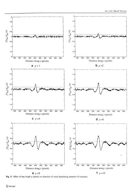
[nt J Adv Manuf Technol2 ,..,--r---~-~-~.'---'-~---'~--'------'---_.----'...-1.51.5--..~ 0.5So...,.:;-l. 0k,~it:; -0.52 0.5So...,.:;I 0---...;1"'-.-0.5-1·1-1.5-1.5-2 '--'--'---'-------'-----'------'----'---'----'-------'--'200 250 300 350 400 450 500 550 600 650Distance along x (pixels)a p= 1-2 '--'__'-_-'----_...L--_---'--_--'-__'-_-'--_--'--_--'---!~ ~ ~ ~ ~ ~ ~ ~ ~ ~Distance along x (pixels)b p=22,..,--r----.---~-....,..-~--r_-_.___-~-~___,1.51.52 0.5""~ I 0---;.,.k,'""'-."- -0.5-1---..k,"-~ I""---.. Ii:~"'-.0.5-1-1.5-2 '--'---'-----'------'------'-------'---'-----'-----'-----'-----'~ ~ ~ ~ ~ ~ ~ ~ ~ BDistance along x (pixels)C p=4-1.5·2 '--'--'----'----'-----'-----'--'----'-------'-----'-------'200 250 300 350 400 450 500 550 600 650Distance along x (pixels)d p=61.51.5---..~ 0.5~'"'P~t;:::: -0.5-1-1-1.5-1.5-2 L2:-':0~0 --:2::-50-=---,3:-':-0~0 --:3::-50.,---4::-00-=---4::-50.,---,5:-':-00.,---,5::-5~0 -6:-':-0-'0-6:-':-50----'Distance along x (pixels)-2 '--'--'----'----'----'---------'---'-----'-----'---.:-':----'200 250 300 350 400 450 500 550 600 650Distance along x (pixels)Fig. 11e p=8Effect of step length p (pixels) on detection of notch (machining duration=20 minutes)f p =10~ Springer
lnt J Adv Manuf Technol1.3I.l0.9j~ 0.70.50.35.2 Application to real imagesMachining duration = 20 min0. I +-........,---,---r--.,..--.,-----,---,---,--.,..--.,----j°Step length P (pixels)Fig. 12 Variation of d(Y)max with step length p10 IIfrom 3 to 25 in odd increments and the difference betweenthe maximum and minimum values of dr.,), i.e., d(x)ma[d(X)lIlif1 was evaluated for each case. Figures 5 (a)-(d)illustrate how d(x) varies with distance along x-directionfor various values of n. Figure 6 shows the variation ofd(x)max-d(X)mif1 with polynomial degree for an unworncutting tool. The polynomial of degree n= 15 was foundto give the smallest value of d(x)max-d(X)min' Thus, thisvalue was used when analyzing worn tools to detect thepresence of notch wear. Since d(x)max=0.137 when n=15for the unworn tool, the threshold for detecting notch wearwas set above this value, i.e., t=0.2. This threshold can beadjusted depending on the minimum size of notch to bedetected.In order to determine the smallest size of notch wear thatcan be detected using the set threshold, notches of varioussizes were generated on an unworn cutting tool using thesoftware tools in Matlab. Figure 7 shows an example ofthe notch generated and the results of detection using thealgorithm developed. The actual area of the notch can bedetermined by subtracting the images of worn and unworncutting tools. The smallest notch that can be detected usingt=0.2 was found to be five pixels. Using a scaling factor of1.88 J.tm x 2.00 J.tm (determined by calibration using pingages), we found that the smallest notch area correspondsto 1.88 x 10- 5 mm 2 . The simulation study was also repeatedby moving the notch to different locations and introducingmore than one notch. In all these cases, the notch defectswere detected successfully.The cutting tools were captured before machining to get theinitial image of tool tip. The cutting speed was initiallyfixed at 134 m/min and other machining conditions areshown in Table I. Images of worn cutting tool tips werecaptured during different time intervals. Figures 8 (a)-(d)show images of the tool at different machining time wherethe growth of notch is clearly visible after 20 minutes ofmachining. Figures 9 (a)-(d) show another set of imagescaptured under a different cutting speed (190 m/min) whereas in the previous case the notch becomes visible after 20minutes. The notch wear location was automaticallydetermined using the algorithm developed in this study.Figure 10 (a) shows the results obtained for a cutting toolafter 40 minutes of machining where the notch has beensuccessfully detected using t=0.2 (cutting speed 134 m/min). Similary, Fig. 10 (c) show the result of notchdetection for the repeated study after 20 minutes ofmachining (cutting speed 190 m/min). The location of thenotch measured in the horizontal direction from the left ofthe image is displayed on the lower left comer of bothimages. From Figs. 10 (b) and (d) the effect of the notch onthe difference d(x) = f'(xm) -.f~p(x) is clearly visible. Anabrupt increase in the value of d(x) can be observed at thenotch. The detection was repeated for other machiningdurations and in all cases the presence of the notch could bedetected. The results for both cutting speeds show that thenotch wear can be detected successfully using the proposedgradient approach.5.3 Effect of changing step length pThe step length was varied from p= 1 to p= 10 pixels tostudy its effect on the ability of the proposed algorithm fordetecting the notch defect. Images of the cutting tool insel1machined for durations of 20 and 40 minutes (Figs. 8 (b)and (d) were used in this study. Figures 11 (a)-(f) show thevariation of the difference f'(xlIl ) -fl/p(x) along the xdirection for machining duration of 20 minutes. For thesame notch size it was found that the maximum differenced(x)l1lax increased with p approximately as a second degreepolynomial function (Fig. 12). Similar trends were observedfor the insert machined for 40 minutes (larger notch wear).From Figs. 11 (a)-(f) a general increase in the waviness ofthe difference plot can be seen as p increases. This is due tothe increase in error when a larger step size is used in thegradient calculation. For the smallest step size ofp= I pixelthe presence of notch can still be detected because themaximum difference d(x)max exceeds the threshold of t=g.2. For a larger step size, e.g., p> 10 pixels, the regionwhere the presence of notch is searched has to be madesmaller, thus missing notches outside this region. Therefore.a value ofp between two to ten pixels is adequate for thedetection of notch defects.6 ConclusionThe gradient detection algorithm with polynomial fittingproposed in the work is able to detect the location of©Springer