COMPUTING

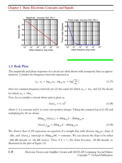
Chapter 1 Basic Electronic Concepts and SignalsMagnitude (dB)0-20-40-60-80Magnitude - low-pass filter, RC=1Phase angle (degrees)Phase angle- low-pass filter, RC=1-40-50-60-70-80-10010 0 10 1 10 2 10 3 10 4 10 5radian frequency (log scale)-9010 0 10 1 10 2 10 3 10 4 10 5radian frequency (log scale)1.5 Bode PlotsThe magnitude and phase responses of a circuit are often shown with asymptotic lines as approximations.Consider two frequency intervals expressed asu 2 – u 1 = log ω – log 10ω 1=10 2ω----- 2ω 1log ⎝⎛ ⎠⎞(1.17)then two common frequency intervals are (1) the octave for whichfor which ω 2 = 10ω 1 .Now, let us consider a circuit whose gain is given asG( ω) v = C ⁄ ω kω 2 = 2ω 1and (2) the decade(1.18)where C is a constant and k is a non−zero positive integer. Taking the common log of (1.18) andmultiplying by 20 we obtain20log { G( ω) v } = 20log C – 20klog ω101010{ G( ω) v } = 20log C – 20klog ωdB 1010(1.19)We observe that (1.19) represents an equation of a straight line with abscissa log 10ω , slope of– 20k , and { G( ω) v } intercept at 20log1010C= constant. We can choose the slope to be either– 20k dB ⁄ decade or – 6k dB ⁄ octave. Thus, if k = 1, the slope becomes – 20 dB ⁄ decade asillustrated in the plot of Figure 1.8.1−8Electronic Devices and Amplifier Circuits with MATLAB Computing, Second EditionCopyright © Orchard Publications