Measurements

Chapter 2: Fundamentals
τ
τ
τ
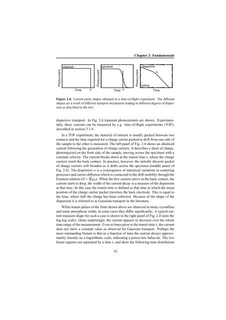
Figure 2.4: Current pulse shapes obtained in a time-of-flight experiment. The different
shapes are a result of different transport mechanism leading to different degrees of dispersion
as described in the text.
dispersive transport. In Fig. 2.4 transient photocurrents are shown. Experimentally,
these currents can be measured by e.g. time-of-flight experiments (TOF),
described in section 3.1.4.
In a TOF experiment, the material of interest is usually packed between two
contacts and the time required for a charge carrier packed to drift from one side of
the sample to the other is measured. The left panel of Fig. 2.4 shows an idealized
current following the generation of charge carriers. It describes a sheet of charge,
photoinjected on the front side of the sample, moving across the specimen with a
constant velocity. The current breaks down at the transit time t τ where the charge
carriers reach the back contact. In practice, however, the initially discrete packet
of charge carriers will broaden as it drifts across the specimen (middle panel of
Fig. 2.4). The dispersion w is a consequence of statistical variations in scattering
processes and carrier diffusion which is connected to the drift mobility through the
Einstein relation (D = kT e µ d). When the first carriers arrive at the back contact, the
current starts to drop, the width of the current decay is a measure of the dispersion
at that time. In this case the transit time is defined as that time at which the mean
position of the charge carrier packet traverses the back electrode. This is equal to
the time, where half the charge has been collected. Because of the shape of the
dispersion it is referred to as Gaussian transport in the literature.
While transit pulses of the form shown above are observed in many crystalline
and some amorphous solids, in some cases they differ significantly. A typical current
transient shape for such a case is shown in the right panel of Fig. 2.4 (note the
log-log scale). Quite surprisingly, the current appears to decrease over the whole
time range of the measurement. Even at times prior to the transit time t τ the current
does not show a constant value as observed for Gaussian transport. Perhaps the
most outstanding feature is that as a function of time the current decays approximately
linearly on a logarithmic scale, indicating a power-law behavior. The two
linear regimes are separated by a time t τ and show the following time distribution
16