Remaining Life of a Pipeline

andom variable with its own degree of variability. This variability is the most important factor when
estimating the remaining life of a pipeline, and the estimation method of such variability is the most
valuable contribution of the proposed approach.
4.2. Methodology
4.2.1 Step #1: Uncertainty Propagation
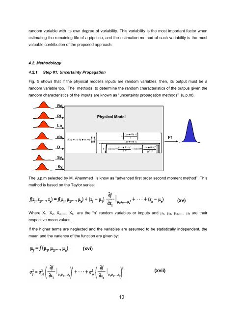
Fig. 5 shows that if the physical model’s inputs are random variables, then, its output must be a
random variable too. The methods to determine the random characteristics of the outpus given the
random characteristics of the imputs are known as “uncertainty propagation methods” (u.p.m).
Rd
Rl
Physical Model
Lo
do
D
pf( t ) 2. ( Sy 68.95)
. T .
D
1
1
( do Rd.
t )
T
( do Rd.
t )
Lo Rl.
T.
( t ) 2
1 0.6275. DT . 0.003375.
( Lo Rl.
t ) 4
D 2 . T 2
Pf
Sy
Sy
fig.5
The u.p.m selected by M. Ahammed is know as “advanced first order second moment method”. This
method is based on the Taylor series:
(xv)
Where X 1 , X 2 , X 3 ,...., X n
respective mean values.
are the “n” random variables or imputs and µ 1 , µ 2 , µ 3 ,...., µ n are their
If the higher terms are neglected and the variables are assumed to be statistically independent, the
mean and the variance of the function are given by:
(xvi)
(xvii)
10